RPA in Yambo: local field effects¶

In this tutorial you will learn how to calculate the macroscopic dielectric function with Yambo using two-dimensional (2D) hBN as an example.

Requirements

SAVE folder of 2D hBN: download and extract hBN-2D.tar.gz from the Tutorial files page
yambo executable
gnuplot for plotting spectra

It is assumed that you are familiar with the concepts related to the SAVE folder and handling files with Yambo.

See also

Optics at the independent particle level

The macroscopic dielectric function is obtained by including the so called local field effects (LFE) in the calculation of the response function.

Within the time-dependent DFT formalism this is achieved by solving the Dyson equation for the susceptibility \(\chi\). In reciprocal space this is given by:

(1)¶\[\chi_{\mathbf{G}, \mathbf{G}^{\prime}}(\mathbf{q}, \omega) = \chi_{\mathbf{G}, \mathbf{G}^{\prime}}^{0}(\mathbf{q}, \omega)+\sum_{\mathbf{G}_{1}, \mathbf{G}_{2}} \chi_{\mathbf{G}, \mathbf{G}_{1}}^{0}(\mathbf{q}, \omega) \left[ v_{\mathbf{G}_{1}}(\mathbf{q}) \delta_{\mathbf{G}_{1}, \mathbf{G}_{2}}+f_{\mathbf{G}_{1}, \mathbf{G}_{2}}^{x c} \right] \chi_{\mathbf{G}_{2}, \mathbf{G}^{\prime}}(\mathbf{q}, \omega) \, .\]

The microscopic dielectric function is related to \(\chi\) by

(2)¶\[\epsilon_{\mathbf{G}, \mathbf{G}^{\prime}}^{-1}(\mathbf{q}, \omega) = \delta_{\mathbf{G}, \mathbf{G}^{\prime}} + v_{\mathbf{G}}(\mathbf{q}) \chi_{\mathbf{G}, \mathbf{G}^{\prime}}(\mathbf{q}, \omega)\]

and the macroscopic dielectric function is obtained by taking the \(\mathbf{G}=\mathbf{G^{\prime}}=0\) component of the inverse microscopic one

(3)¶\[\epsilon_{M}(\mathbf{q},\omega) = \frac{1}{\epsilon_{\mathrm{G}=0, \mathrm{G}^{\prime}=0}^{-1}(\mathbf{q}, \omega)} \, .\]

Experimental observables like the optical absorption and the electron energy loss are obtained from the macroscopic dielectric function. The optical absorption is in particular defined in the optical limit:

(4)¶\[\operatorname{Abs}(\omega) = \lim_{\mathbf{q} \rightarrow 0} \operatorname{Im} \epsilon_{M}(\mathbf{q},\omega)=\lim_{\mathrm{q} \rightarrow 0} \frac{1}{\epsilon_{\mathrm{G}=0, \mathrm{G}^{\prime}=0}^{-1}(\mathbf{q}, \omega)} \ \]

The electron energy loss, on the other hand, can be probed in experiments even outside of the optical limit:

(5)¶\[\operatorname{EELS}(\mathbf{q},\omega) = -\operatorname{Im} \frac{1}{\epsilon_{M}(\mathbf{q},\omega)} = -\epsilon_{\mathrm{G}=0, \mathrm{G}^{\prime}=0}^{-1}(\mathbf{q}, \omega).\]

In the following we will neglect the \(f_{\mathbf{G}_1,\mathbf{G}_2}^{xc}\) term in the kernel: we perform the calculation at the RPA level including just the Hartree term (from \(v_G\)).

If we also neglect the Hartree term we go back to the independent particle approximation since we effectively remove the kernel and set \(\chi = \chi_0\).

Before starting go to the hBN-2D/YAMBO directory and initialize the SAVE folder:

$ cd hBN-2D/YAMBO
$ ls
SAVE
$ yambo

Input file and parameters¶

After the initialization we can generate the input file. To include the local fields variables use -o c -k hartree. Check the meaning of the options with the command-line interface if you are not familiar with them.

Let’s start doing a calculation with the light polarization \(\mathbf{q}\) in the plane of the BN sheet. Generate the input like this

$ yambo -F yambo.in_RPA -V RL -o c -k hartree

(thus naming it yambo.in_RPA) and then set the following variables to these values:

 FFTGvecs=  3951            RL       # [FFT] Plane-waves
 Chimod= "Hartree"                   # [X] IP/Hartree/ALDA/LRC/BSfxc
 NGsBlkXd=  3        Ry              # [Xd] Response block size
 % QpntsRXd
  1 | 1 |                            # [Xd] Transferred momenta
 %
 % EnRngeXd
  0.00000 | 20.00000 | eV            # [Xd] Energy range
 %
 % DmRngeXd
  0.20000 | 0.200000 | eV            # [Xd] Damping range
 %
 ETStpsXd= 2001                      # [Xd] Total Energy steps
 % LongDrXd
 1.000000 | 0.000000 | 0.000000 |    # [Xd] [cc] Electric Field
 %

In this input file:

We evaluate the \(\mathbf q \to 0\) response function choosing the direction in the limit parallel to the plane of the hBN sheet;
We set the energy range for the spectrum to \(0-20\) eV;
We set the broadening through the variable DmRngeXd;
We select the Hartree kernel;

Note

While FFTGvecs controls the cutoff for the plane wave expansion of the wavefuntions (hidden in dipole matrix elements appearing in the expression of \(\chi_0\)), NGsBlkXd determines the size of the dielectric matrix in G-space (or equivalently the cutoff on the sum over \(\mathbf{G}_1, \mathbf{G}_2\) in Eq. (1)). Remember that NGsBlkXd is a typical parameter to be converged while it is better to not modify FFTGvecs and leave it at its default (maximum) value.

LFE in the periodic direction¶

../../_images/hBN-2D-3x3.png — Atomic structure of 2D hBN (\(z \parallel c\) is the non-periodic direction).¶

Let’s now run the calculation choosing an appropriate job string label, e.g. one that specifies the electric field direction:

$ yambo -F yambo.in_RPA -J q100

This calculation should take a couple of minutes in serial.

Let’s now look at the results. We want to compare the absorption with and without the local fields: by inspecting the output file o-q100.eps_q1_inv_rpa_dyson we find that this information is given in the 2\(^{nd}\) and 4\(^{th}\) columns, respectively:

$ head -n 50 o-q100.eps_q1_inv_rpa_dyson | grep '#' | tail -n 3
#
#    E[1] [eV]          Im(eps)            Re(eps)            Im(eps_o)          Re(eps_o)
#

Plot the RPA and the IPA response:

 $ gnuplot
 $ gnuplot> plot "o-q100.eps_q1_inv_rpa_dyson" u 1:2 w l t "RPA-LFE","o-q100.eps_q1_inv_rpa_dyson" u 1:4 w l t "noLFE", "o-q100.eel_q1_inv_rpa_dyson" u 1:4 w l ls 7 dt 2 t "EELS"

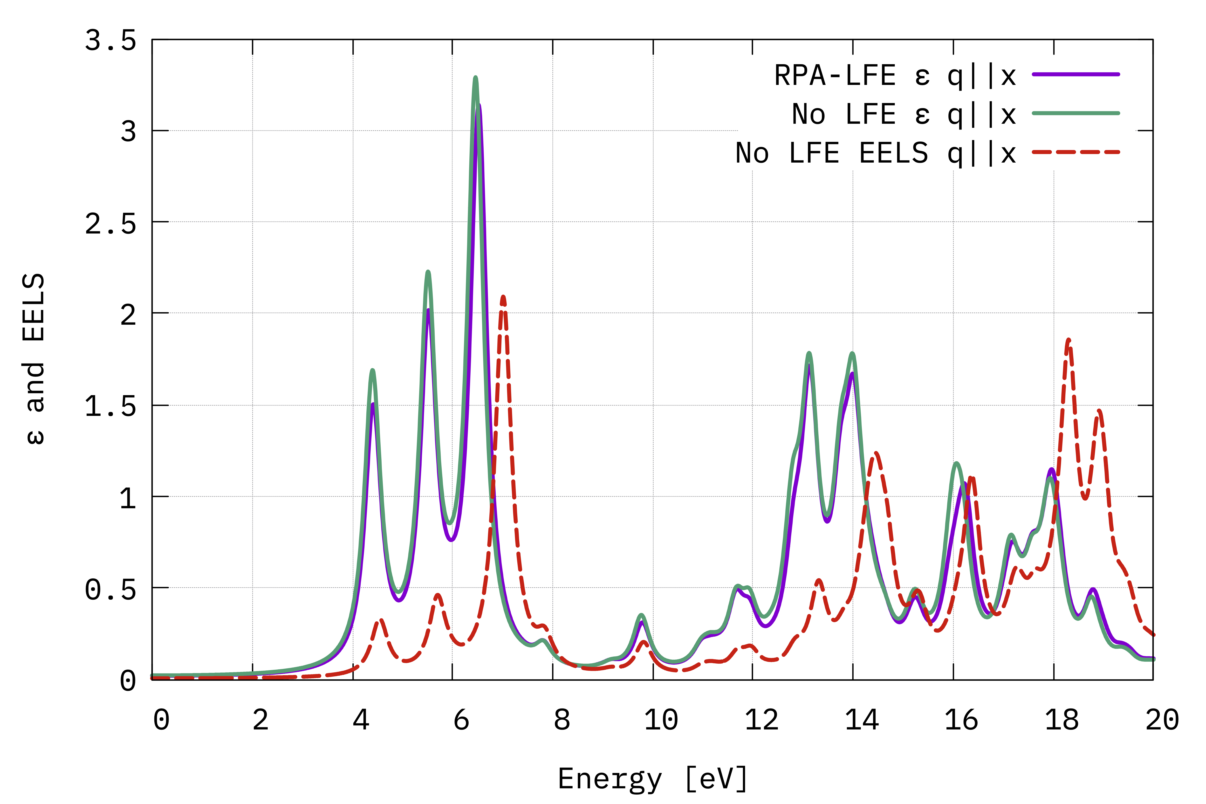
../../_images/hBN-2D-LFE_qx.png — Absorption and EELS spectra (in the optical limit) from the macroscopic dielectric function (Eq. (4) and Eq. (5)) with the electric field in the in-plane direction.¶

There is very little influence of local fields for 2D hBN. This is generally the case for semiconductors or materials with a smoothly varying electronic density.

In the same figure, we have also shown the EELS spectrum (o-q100.eel_q1_inv_rpa_dyson) for comparison.

LFE in the non-periodic direction¶

Now let’s orientate \(\mathbf{q}\) in the direction perpendicular to the BN plane. Open the input file yambo.in_RPA and change LongDrXd to:

% LongDrXd
0.000000 | 0.000000 | 1.000000 |        # [Xd] [cc] Electric Field
%

Run the calculation (don’t forget to change the -J label):

$ yambo -F yambo.in_RPA  -J q001 >& /dev/null &

The >& /dev/null & makes Yambo run in the background and print the log into a file. You can follow the progress of the calculation with

$ tail -f l-q001_optics_dipoles_kernel_chi

When the calculation is done we can plot the new output:

$ gnuplot
gnuplot> plot "o-q001.eps_q1_inv_rpa_dyson" u 1:2 w l,"o-q001.eps_q1_inv_rpa_dyson" u 1:4 w l

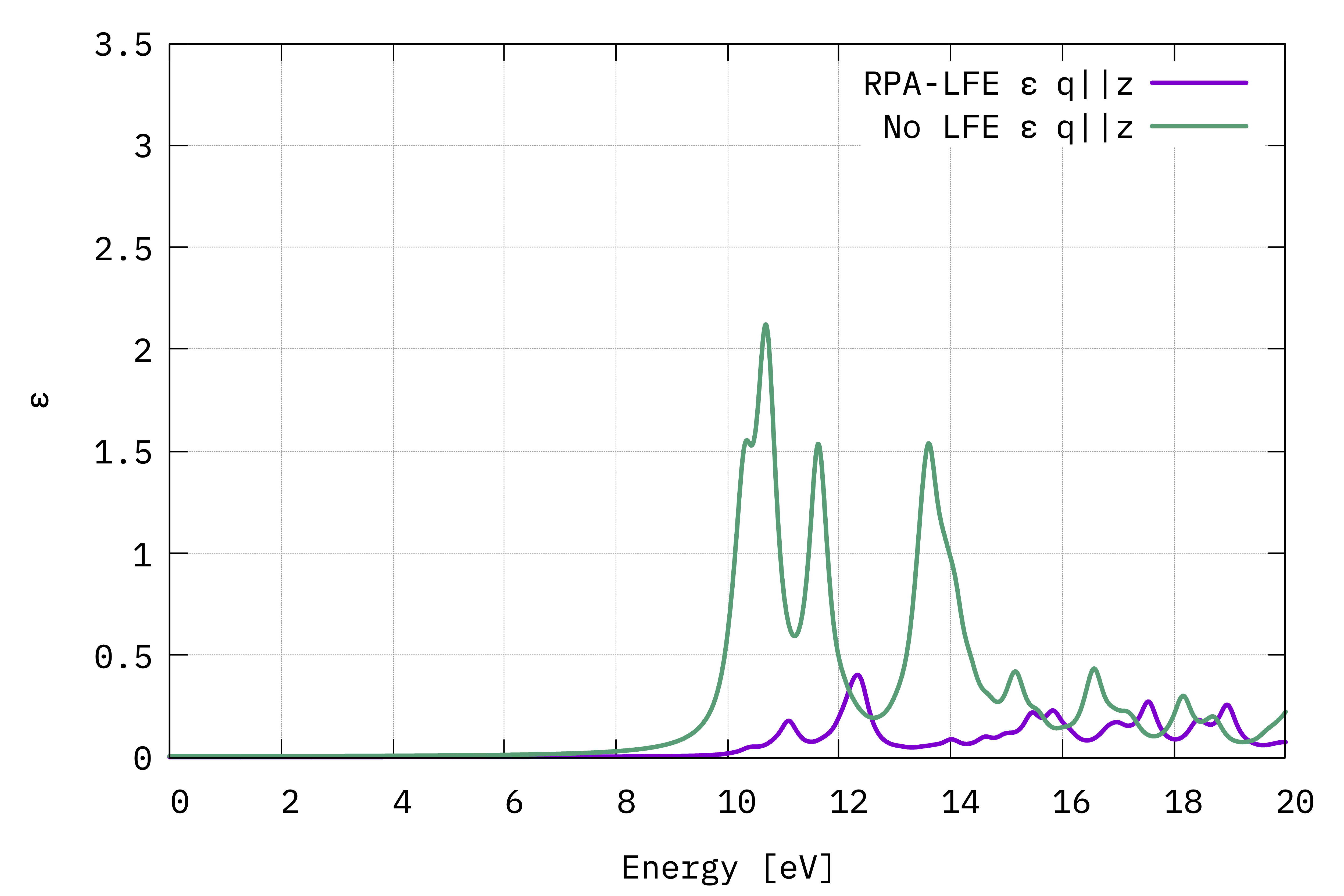
../../_images/hBN-2D-LFE_qz.png — Absorption spectra from the macroscopic dielectric function (Eq. (4)) with the electric field in the out-of-plane direction.¶

In the out of plane direction, the absorption is strongly blueshifted with respect to the in-plane absorption. Furthermore, the influence of local fields is striking and quenches the spectrum strongly. This is the well known depolarization effect.

Local field effects are much stronger in the perpendicular direction because the charge inhomogeneity is dramatic. Also keep in mind that many G-vectors are needed to account for the sharp change in the potential across the BN-vacuum interface.

Absorption vs EELS¶

In order to understand this further, we plot the electron energy loss spectrum for this component and compare with the absorption:

$ gnuplot
$ gnuplot > plot "o-q001.eps_q1_inv_rpa_dyson" w l,"o-q001.eel_q1_inv_rpa_dyson" w l

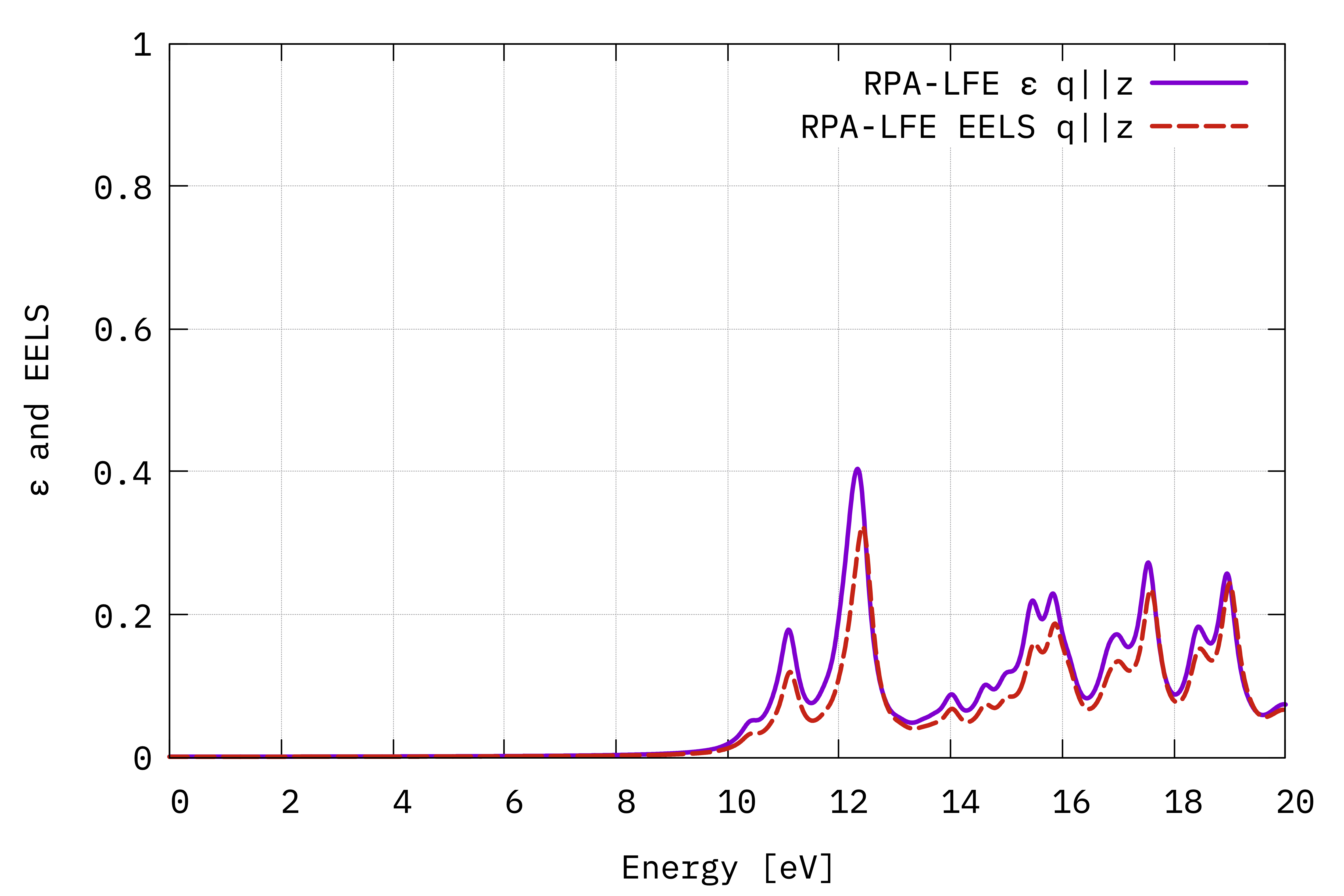
../../_images/hBN-2D-LFE_qz_abs-vs-eels.png — Absorption and EELS spectra (in the optical limit) from the macroscopic dielectric function (Eq. (4) and Eq. (5)) with the electric field in the out-of-plane direction.¶

The conclusion is that the absorption and EELS coincide for isolated systems. To understand this result, you need to consider the role of the macroscopic screening in the response function and the long-range part of the Coulomb potential. See e.g. this article [2]

Note

In order to have exactly coinciding EELS and absorption spectra here, we actually need to include the truncation of Coulomb interaction (using the -r flag when generating the input). The Coulomb cutoff is needed because we did not include enough vacuum along the non-periodic stacking direction, which results in spurious interactions between periodic replicas. The erroneous difference is proportional to the volume of the unit cell, reflecting the fact that the finite number of \(\mathbf{G}\) vectors along the \(z\) direction (too low since we have not enough vacuum) spoils the value of \(\epsilon_{00}^{-1}\) and eventually also of \(\epsilon_{00}\) after the inversion. With the Coulomb cutoff, instead, the \(\mathbf{G}\) vectors along \(z\) are effectively continuous (as it is equivalent to having infinite vacuum).

Finally, notice that when you use the Coulomb cutoff Yambo does not produce two different output files o.eps_* and o.eel_*, but a single output file o.alpha_*: the correct physical quantity to calculate in 2D is the 2D polarisability.

EELS Dispersion (optional)¶

We can also calculate the EELS dipersion by performing the RPA calculations at finite momenta \(\mathbf{q}\).

Note

To clearly see the EELS dispersion we need to increase the k-points sampling of the Brillouin zone. For the results shown in the following, we increased the grid to \(18 \times 18 \times 1\) and the cutoff for the dielectric matrix to 10 Ry. Be aware that this makes the calculation much heavier, so you might want to use different parameters (k-point grid, energy cutoff, number of bands…) to be able to run it on your machine.

To do this we increase the range of calculated \(\mathbf{q}\) points via QpntsRXd and it is sufficient to focus on a narrower energy window. We also want to include the cutoff of the Coulomb interaction for 2D materials, so generate a new input file with

$ yambo -F yambo.in_eels -r -o c -k hartree

and change the highlighted input variables as shown here:

[...]
rim_cut                          # [R] Coulomb potential
chi                              # [R][CHI] Dyson equation for Chi.
dipoles                          # [R] Oscillator strenghts (or dipoles)
[...]
RandQpts=1000000                 # [RIM] Number of random q-points in the BZ
RandGvec= 100              RL    # [RIM] Coulomb interaction RS components
CUTGeo= "slab z"                 # [CUT] Coulomb Cutoff geometry: box/cylinder/sphere/ws/slab X/Y/Z/XY..
[...]
Chimod= "HARTREE"                # [X] IP/Hartree/ALDA/LRC/PF/BSfxc
NGsBlkXd= 10               Ry    # [Xd] Response block size
% QpntsRXd
   1 |  6 |                         # [Xd] Transferred momenta
%
% BndsRnXd
   1 |  60 |                         # [Xd] Polarization function bands
%
% EnRngeXd
  3.00000 | 12.00000 |         eV    # [Xd] Energy range
%
% DmRngeXd
 0.200000 | 0.200000 |         eV    # [Xd] Damping range
%
ETStpsXd= 2001                    # [Xd] Total Energy steps
% LongDrXd
 1.000000 | 0.000000 | 0.000000 |        # [Xd] [cc] Electric Field
%

In this way, we will find the EELS spectra for a finite number of \(\mathbf{q}\) vectors along the \(\Gamma-M\) direction.

Now run the calculation:

$ yambo -F yambo.in_RPA -J eels -C eels.out

We can finally plot the spectra, which are now printed in the files o-eels.alpha_q1_inv_rpa_dyson, o-eels.alpha_q2_inv_rpa_dyson and so on (there are no longer o.eps* and o.eel* files because we used the Coulomb cutoff). Notice that here we plot the normalized EELS dispersion, as generally EELS spectra have very different intensities at different \(\mathbf{q}\). You can use the provided plt_eels.gnu script.

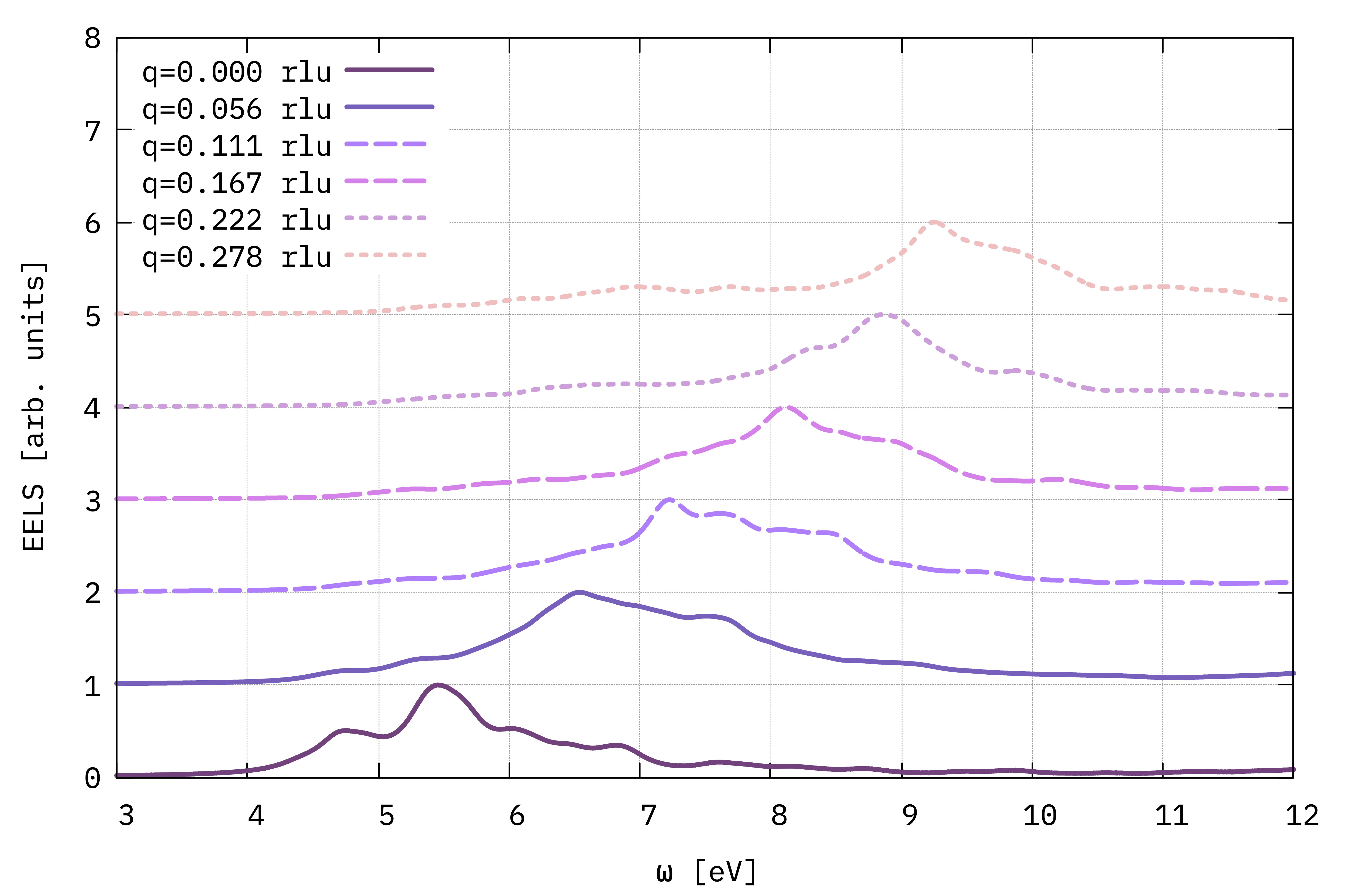
../../_images/hBN-2D-LFE_eels-dispersion.png — Dispersion in momentum of the EELS spectra for \(\mathbf{q}\) along the \(\Gamma-M\) direction, calculated from the macroscopic dielectric function (Eq. (5)).¶

Despite not being fully at convergence, we can already draw conclusions on the typical result of a EELS spectra. This in particular gives access to the evolution with respect to the \(\mathbf{q}\) of the neutral excitations of a material. In the figure shown just above, by following the position in energy of the main peaks we can observe the dispersion in energy of the first allowed single-particle transitions of 2D h-BN.

An EELS spectrum can also provide information on the charge neutral excitations of a material, the plasmons, which are the peaks found in correspondence of \(\text{Re} \epsilon_M=0\).