Hartree-Fock on hBN

In this tutorial you will learn how to calculate the quasiparticle corrections in the Hartree-Fock (HF) approximation and how to choose the related input parameters to obtain meaningful converged results. We will use bulk hBN as an example system.

Requirements

• SAVE folder of bulk hBN: download and extract hBN.tar.gz from the Tutorial files page

• yambo executable

• gnuplot for plotting the results

In general we want to obtain quasiparticle correction to energy levels using many-body perturbation theory (MBPT). The general non-linear quasiparticle equation reads:

\[E_{n\boldsymbol{k}}^{\mathrm{QP}} = \varepsilon_{n\boldsymbol{k}} + \langle \psi_{n\boldsymbol{k}} | \Sigma(E_{n\boldsymbol{k}}^{\mathrm{QP}}) - V_{xc} | \psi_{n\boldsymbol{k}} \rangle \, ,\]

where \(E_{n\boldsymbol{k}}^{\mathrm{QP}}\) are the quasiparticle-corrected energies, \(\varepsilon_{n\boldsymbol{k}}\) and \(\psi_{n\boldsymbol{k}}\) are the DFT energies and wavefunctions, \(V_{xc}\) the DFT exchange-correlation potential and \(\Sigma\) the self-energy.

In practice, what Yambo does is to compute the self-energy to obtain the corrections to the one-particle (Kohn-Sham DFT) energies. In the GW approach the self-energy can be separated into two components: a static term called the exchange self-energy (\(\Sigma^x\)), and a dynamical term (energy dependent) called the correlation self-energy (\(\Sigma^c\)), that is

\[\Sigma_{n\boldsymbol{k}}(\omega) = \Sigma_{n\boldsymbol{k}}^x + \Sigma_{n\boldsymbol{k}}^c(\omega) \, .\]

In this tutorial we only consider the exchange self-energy and compute the corresponding quasiparticle energies, which basically consists in a HF calculation.

In reciprocal space the exchange part contribution to the self-energy for a generic state (\(n\boldsymbol{k}\)) reads

(1)\[\Sigma_{n\boldsymbol{k}}^x = \langle n\boldsymbol{k} | \Sigma^x | n\boldsymbol{k} \rangle = - \sum_m \int_{\mathrm{BZ}} \frac{d\boldsymbol{q}}{(2\pi)^3} \sum_{\boldsymbol{G}} v(\boldsymbol{q}+\boldsymbol{G}) |\rho_{nm}(\boldsymbol{k},\boldsymbol{q},\boldsymbol{G})|^2 f_{m\boldsymbol{k-q}} \, ,\]

where \(v\) is the Coulomb potential, \( \rho_{mn}(\boldsymbol{k},\boldsymbol{q},\boldsymbol{G}) =\langle n\boldsymbol{k} | e^{i(\boldsymbol{q}+\boldsymbol{G})\cdot\boldsymbol{r}} | m\boldsymbol{k-q}\rangle \) are the dipole matrix elements and \(f\) are the occupation factors.

Note

In this way we are adding the HF contribution in a perturbative way to previously calculated DFT energies, i.e.

(2)\[E_{n\boldsymbol{k}}^{\mathrm{HF}} = \varepsilon_{n\boldsymbol{k}}^{\mathrm{DFT}} + (\Sigma_{n\boldsymbol{k}}^x - V_{n\boldsymbol{k}}^{xc}) \, ,\]

so they will differ from a standard self-consistent HF calculation.

Before starting go to the hBN/YAMBO directory and initialize the SAVE folder:

$ cd hBN/YAMBO
$ ls
SAVE
$ yambo

Input file and variables

Let’s start by building up an input file for a HF calculation. From yambo -h we can see that the option to be used is -hf (or -x):

$ yambo -x -F hf.in

The input file hf.in contains the following variables:

HF_and_locXC                     # [R] Hartree-Fock
EXXRLvcs=  3187            RL    # [XX] Exchange    RL components
VXCRLvcs=  3187            RL    # [XC] XCpotential RL components
%QPkrange                        # [GW] QP generalized Kpoint/Band indices
1|14|1|100|
%

Note

HF_and_locXC is a runlevel variable (marked with [R]). These variables tell Yambo which parts of the code should be executed. Each runlevel enables its own set of input variables. In particular HF_and_locXC is needed to compute \(\Sigma^x\).

• The variable EXXRLvcs controls the number of G vectors to be summed in the expression of the exchange self-energy (see Eq.(1)).

• The variable VXCRLvcs sets the number of G vectors used in the evaluation of the density for the \(V_{xc}\) matrix element.

  Important

  A large number of G vectors is needed in order to have a precise cancellation with the ground state calculation, in particular when GGA potentials are used. A good practice is to leave VXCRLvcs at the maximum number (default)[1].

  Also notice that \(\Sigma_{n\boldsymbol{k}}^x\) and \(V_{n\boldsymbol{k}}^{xc}\) are to be subtracted, it is important to keep the same value of EXXRLvcs and VXCRLvcs in order to compute them with the same accuracy.

  In this tutorial we will ignore these recommendations just to show the convergence behaviour of a HF calculation.

• The QPkrange name list it is a generalized index needed to select the first and last kpoints as well as the bands for which we want to calculate the QP correction.

In general, we do not want to calculate the corrections for the entire band structure, but instead we are interested in the gap of the system or in the energies around the Fermi level.

Let’s start by editing the hf.in file by selecting the last occupied and first unoccupied bands. Looking into the r_setup file we find that these are the bands number 8 and 9, so we set the QPkrange variable to

%QPkrange
1|14|8|9|
%

Tip

If you want to compute the quasiparticle correction for only one eigenvalue, for example the one with band index 22 and k point number 3, set

%QPkrange
3|3|22|22|
%

If you want to compute two specific direct gaps between bands 8 and 9 located at k points 7 and 10, set

%QPkrange
7|7|8|9|
10|10|8|9|
%

In the expression of the exchange self-energy (Eq.(1)), we have a summation over bands, an integral over the Brillouin Zone and a sum over the G vectors.

The presence of the occupation factors \(f\) imply that only occupied states enter in the expression, so we do not need to worry about the bands as Yambo will include all the occupied bands by default and thus the sum over \(m\) is automatically restricted to valence bands only.

We can however study the convergence of the G vectors sum. In the following we will perform different calculations varying the kinetic energy cutoff governing the number of G vectors entering the sum.

Calculations

Let’s start by setting

EXXRLvcs= 10 Ry

in hf.in. Now run the calculation with

$ yambo -F hf.in -J 3D

HF_and_locXC log

  __ __  ____ ___ ___ ____   ___
 |  |  |/    |   |   |    \ /   \
 |  |  |  o  | _   _ |  o  )     |
 |  ~  |     |  \_/  |     |  O  |
 |___, |  _  |   |   |  O  |     |
 |     |  |  |   |   |     |     |
 |____/|__|__|___|___|_____|\___/


 <---> [01] MPI/OPENMP structure, Files & I/O Directories
 <---> MPI Cores-Threads   : 1(CPU)-48(threads)
 <---> [02] CORE Variables Setup
 <---> [02.01] Unit cells
 <---> [02.02] Symmetries
 <---> [02.03] Reciprocal space
 <---> [02.04] K-grid lattice
 <---> Grid dimensions      :   6   6   2
 <---> [02.05] Energies & Occupations
 <---> [03] Transferred momenta grid and indexing
 <---> [04] Local Exchange-Correlation + Non-Local Fock
 <---> [FFT-HF/Rho] Mesh size:   18   18   44
 <---> EXS |########################################| [100%] --(E) --(X)
 <---> [xc] Functional : Slater exchange(X)+Perdew & Zunger(C)
 <---> [xc] LIBXC used to calculate xc functional
 <---> [04.01] Hartree-Fock occupations report
 <---> [05] Timing Overview
 <---> [06] Memory Overview
 <---> [07] Game Over & Game summary

Let’s inspect the output file o-3D.hf and the report file r-3D_HF_and_locXC. In the output we have:

v5

$ grep -A7 '#    K-point' o-3D.hf

grep output

#    K-point            Band               Eo [eV]            Ehf [eV]           Vxc [eV]           Vnlxc [eV]
#
        1                   8                -1.296420          -4.793192          -18.03349          -21.53026
        1                   9                 4.832399           9.755576          -9.592623          -4.669446
        2                   8                -1.335510          -4.809560          -18.07514          -21.54919
        2                   9                 7.567424           13.43130          -11.55020          -5.686331
        3                   8                -2.259589          -6.012086          -17.72660          -21.47909
        3                   9                 5.775240           10.83750          -9.685234          -4.622970
...

v4.5 (or older)

$ grep -A7 '#    K-point' o-3D.hf

grep output

#  K-point          Band       Eo           Ehf        Vxc (DFT)   Vnlxc (HF)
#
    1.00000      8.00000     -1.29642     -4.79324    -18.03344    -21.53026
    1.00000      9.00000      4.83239     9.755507    -9.592554    -4.669446
    2.00000      8.00000     -1.33551     -4.80994    -18.07476    -21.54919
    2.00000      9.00000      7.56742     13.43122    -11.55012    -5.686330
...

Looking at the definition of the HF energy (Eq.(2)), the third column (Eo) is the DFT eigenvalue, Ehf is the HF energy, while columns 5 and 6 report the two different contributions to the unperturbed DFT eigenvalue: Vxc (i.e. \(V_{n\boldsymbol{k}}^{xc}\) to be subtracted) and Vnlxc (i.e. \(\Sigma_{n\boldsymbol{k}}^x\) to be added).

From these data we can calculate the HF gap. In the report file we find that the direct gap is located at k-point number 7 and its value is 4.29 eV at DFT level and 11.95 eV in the HF approximation.

Tip

These values are printed in their respective sections of the report file: Energies & Occupations for DFT and Hartree-Fock occupations report for HF.

$ grep "Direct Gap" r-3D_HF_and_locXC
[X] Direct Gap                                    :  4.289853 [eV]
[X] Direct Gap localized at k                     :   7
[Hartree-Fock] Direct Gap                         :  11.94549 [eV]
[Hartree-Fock] Direct Gap localized at k          :   7

Convergence of the direct gap

In order to converge the direct gap we will focus the k point where it is located. Inspecting either the setup report file or any other report file we can see that the direct minimum gap is found at the k-point number 7.

Note

In this example of bulk hBN the 7-th k point corresponds to the M point: you can see this by searching the DFT “Direct Gap” and looking at the eigenvalues reported for each k point. Remember that the zero of the energy is fixed at the top of the valence band, which in this case is located at the k point number 14 (H point).

Thus we restrict the convergence calculations to the occupied and empty bands at point M by modifying QPkrange in the input file as follows:

%QPkrange
7|7|8|9|
%

Tip

Even if in this example the calculations are not at all expensive, reducing the calculations to few bands when performing convergence tests allows to save memory and time.

We now run a series of calculations changing the value of EXXRLvcs, let’s say to 10, 20, 30 and 40 Ry. Create four different input files which only differ for the EXXRLvcs value and name them hf_10Ry.in, hf_20Ry.in, etc.

$ cp hf.in hf_10Ry.in
$ cp hf.in hf_20Ry.in
...

After you have set EXXRLvcs to the corresponding value in each hf_*.in file, run the calculations one by one:

$ yambo -F hf_10Ry.in -J 3D
$ yambo -F hf_20Ry.in -J 3D
...

Once you have run all the calculations collect the results found in the output files, for example putting in a file named hf.dat the following data: cutoff energy (10, …, 40 Ry), number of G vector in the sum (found in the report), HF energy for the occupied state (Ehf for band 8), HF energy for the unoccupied state (Ehf for band 9).

You can use these two grep commands to extract Ehf for band 8

$ grep "^ *7 *8" o-3D.hf_* | awk '{print $5}'
-2.870097
-3.308719
-3.402065
-3.433922 

and band 9

$ grep "^ *7 *9" o-3D.hf_* | awk '{print $5}'
9.075388
9.018848
9.012869
9.011314

and the following one to extract the number of G vectors

$ grep '  Exchange RL vectors' r-3D_HF_and_locXC_0* | awk '{print $6}'
151
371
651
1009

Your hf.dat file should look like this:

# Energy cutoff [Ry]     N. G vectors     Ehf_8 [eV]     Ehf_9 [eV]
  10                     151              -2.870097      9.075388
  20                     371              -3.308719      9.018848
  30                     651              -3.402065      9.012869
  40                     1009             -3.433922      9.011314

You can plot the results like this

$ gnuplot
gnuplot> plot "hf.dat" u 1:($4-$3)  w lp t "HF gap vs Energy cutoff"
gnuplot> plot "hf.dat" u 2:($4-$3)  w lp t "HF gap vs Number of G vector"

or use a slightly more fancy gnuplot script

set key c

set grid y
set grid x

set xtics nomirror
set x2tics
set xlabel "Cutoff energy [Ry]"
set x2label 'Number of RL vectors in {/Symbol S}^x'
set ylabel "HF direct gap [eV]"

plot "hf.dat" u 1:($4-$3):x2tic(2) w p pt 7 ps 1 t ""
rep  "hf.dat" u 1:($4-$3)          w lp lw 3 pt 7 ps 2 lc 'red' t "HF gap"

(put these lines in a hf.gnu file and then type load 'hf.gnu' in gnuplot).

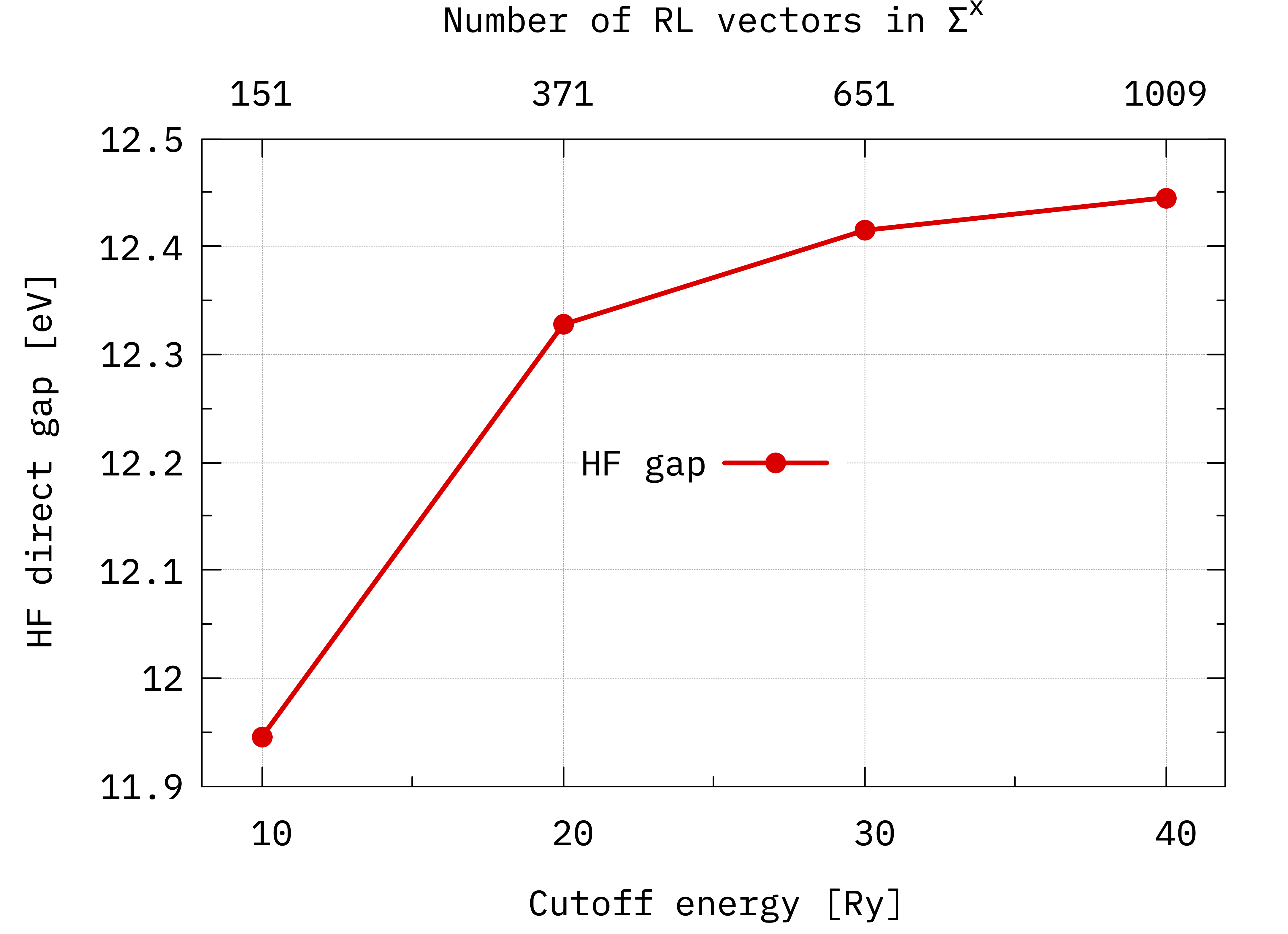
Convergence of the Hartree-Fock direct gap of bulk hBN with respect to the cutoff on the sum over G vectors (see Eq.(1)).

You can see that at 40 Ry the energy gap is very close to convergence. If you plot the occupied and unoccupied bands separately you can see that for this system the unoccupied band converges much faster than the occupied one.

k points convergence (optional)

The last important convergence test deals with the accuracy of the integral over the Brillouin zone in the expression of the Exchange Self-Energy (Eq.(1)), which translates into k point convergence.

To test the convergence with respecto to the k point sampling, you should:

1. Perform a new non-scf calculation with a bigger k point grid;

2. Convert wave functions and electronic structure to Yambo databases in a different directory;

3. Initialize the new Yambo databases;

4. Redo the steps explained in this tutorial for each k point grid.

---

[1]

In case you need to reduce VXCRLvcs (e.g. for memory reason), the accuracy can be checked by comparing the E_xc values printed in the Yambo report file with those from the DFT calculation (usually printed in the output file).