GW on hBN
In this tutorial you will learn how to calculate the quasiparticle corrections in the GW approximation and how to choose the related input parameters to obtain meaningful converged results. We will use bulk hBN as an example system.
Requirements
SAVEfolder of bulk hBN: download and extracthBN.tar.gzfrom the Tutorial files pageyamboexecutableyppexecutablegnuplotfor plotting the results
It is assumed that you are familiar with the concepts related to the SAVE folder and handling files with Yambo.
See also
As we have seen in the Hartree-Fock tutorial, we want to use many-body perturbation theory (MBPT) to calculate quasiparticle energies of materials. This is often done perturbatively on top of the results of a Kohn-Sham DFT calculation:
where \(E_{n\boldsymbol{k}}^{\mathrm{QP}}\) are the quasiparticle-corrected energies, \(\varepsilon_{n\boldsymbol{k}}\) and \(\psi_{n\boldsymbol{k}}\) are the DFT energies and wavefunctions, \(V_{xc}\) the DFT exchange-correlation potential and \(\Sigma\) the self-energy.
We already saw that the GW self-energy can be split into two components, the static exchange term \(\Sigma^x\) and the correlation part \(\Sigma^c\), encompassing the frequency dependence:
In this tutorial we turn our attention to the more demanding dynamical part of the self-energy \(\Sigma_{n\boldsymbol{k}}^c(\omega)\) and see how to determine quasi-partice corrections in the GW approximation.
The correlation part of the self-energy for a generic state \(| n\boldsymbol{k} \rangle\) reads in a plane wave representation:
where \(\rho_{mn}(\boldsymbol{k},\boldsymbol{q},\boldsymbol{G}) =\langle n\boldsymbol{k} | e^{i(\boldsymbol{q}+\boldsymbol{G})\cdot\boldsymbol{r}} | m\boldsymbol{k-q}\rangle\) are the dipole matrix elements, \(G^{0}_{m\boldsymbol{k}}(\omega)\) is the single-particle propagator and \(W_{\boldsymbol{G}\boldsymbol{G'}}(\omega)=v(\boldsymbol{q}+\boldsymbol{G})\epsilon^{-1}_{\boldsymbol{G}\boldsymbol{G'}}(\omega)\) is the screened potential given by the product between the bare Coulomb potential and the inverse dielectric matrix.
In the GW approximation, the inverse dielectric matrix \(\epsilon^{-1}_{\boldsymbol{G}\boldsymbol{G'}}(\omega)\) is calculated at RPA level, which we need to evaluate including the local field effects as discussed in the RPA-LFE tutorial.
Concerning the single-partile propagator \(G^{0}_{m\boldsymbol{k}}(\omega)\), the time-ordered representation is employed:
where \(\mu\) is the chemical potential or Fermi level.
Note
The poles of \(G^{0}_{m \boldsymbol{k}}(\omega)\) in eq (4) have opposite sign of the imaginary part for occupied and empty states.
In Yambo, you can set set the distance of single-particle poles from the real
axis through the variable GDamping.
Focusing now more in depth on the expression of the correlation self energy in Eq (3) we see that it is rather complicated. It features:
a summation over bands
an integral over the Brillouin Zone
a sum over the G vectors
an integral in frequency
Important
In contrast to the case of \(\Sigma^{x}\), here the summation over bands extends over all bands (including unoccupied ones), and so convergence tests of the number of bands included in the sum are needed.
Another important difference is that Eq (3) features the screened interaction \(W\), that needs to be properly evaluated not just regarding the number of G vectors but also in its frequency dependence.
Different methods to describe the frequency dependence of \(W_{\boldsymbol{G}\boldsymbol{G'}}(\omega)\) are available in Yambo.
In this tutorial, we will perform GW calculation under a simplified but widely used approximation called the plasmon pole approximation (PPA): In this approximation the frequency dependence of each component of \(W_{\boldsymbol{G}\boldsymbol{G'}}(\omega)\) is represented through a single pole function.
Note
Different methods to describe the frequency dependece of \(W\) are presented in this tutorial.
For now, keep in mind that the PPA is a reasonable approximation for semiconductors and insulators.
PPA in a nutshell
The basic idea of the plasmon-pole approximation is to describe the frequency dependence of the inverse dielectric matrix with a single-pole function of the form:
The two parameters \(R_{\boldsymbol{G}\boldsymbol{G'}}\) and \(\Omega_{\boldsymbol{G}\boldsymbol{G'}}\) are obtained by a fit (for each component) after calculating the RPA dielectric matrix explicitely at two given frequencies.
Attention
Yambo by default calculates the dielectric matrix in the static limit (\(\omega=0\)) and at a user defined frequency called the plasmon-pole frequency (\(\omega=i \omega_p\)).
The PPA approximation has the great computational advantage of calculating the dielectric matrix only for two frequencies and allows for an analytical expression of the frequency integral in Eq (3).
Once the correlation part of the self-energy is calculated, we can go back to calculate the quasi-particle energies. This is not straightforward as the quasi-particle energies are determined self-consistently in Eq (1), which in general is non-linear.
In the following, unless otherwise stated, we will solve the non-linear quasi-particle equation at first order by expanding the self-energy around the Kohn-Sham eigenvalues. In this way the quasiparticle equation reads:
where the normalization factor \(Z_{n\boldsymbol{k}}\) is defined as:
We can now proceed to perform a GW calculation. In the following, we will first familiarize with the results of a GW calculation in Yambo and then check the convergence of the quasiparticle energies with respect to the different parameters appearing in Eq.(3).
Go to the hBN/YAMBO directory and initialize the SAVE folder:
$ cd hBN/YAMBO
$ ls
SAVE
$ yambo
Input file generation
Let’s begin by creating an input file for a GW PPA calculation.
This also includes the variables to calculate the exchange part
of the self-energy.
As usual you can use yambo -h to determine the right options.
To generate the correct input in this case type:
$ yambo -hf -gw0 ppa -dyson n -F gw_ppa.in
(or yambo -x -p p -g n -F gw_ppa.in in compact form).
Edit the generated input file in the following way:
HF_and_locXC                        # [R XX] Hartree-Fock Self-energy and Vxc
ppa                                 # [R Xp] Plasmon Pole Approximation
gw0                                 # [R GW] GoWo Quasiparticle energy levels
em1d                                # [R Xd] Dynamical Inverse Dielectric Matrix
EXXRLvcs = 40          Ry           # [XX] Exchange RL components
VXCRLvcs = 3187        RL           # [XC] XCpotential RL components
Chimod= "Hartree"                   # [X] IP/Hartree/ALDA/LRC/BSfxc
% BndsRnXp
  1 | 10 |                          # [Xp] Polarization function bands
%
NGsBlkXp = 1            Ry          # [Xp] Response block size
% LongDrXp
 1.000000 | 1.000000 | 1.000000 |   # [Xp] [cc] Electric Field
%
PPAPntXp = 27.21138    eV           # [Xp] PPA imaginary energy
%GbndRnge
  1 | 40 |                          # [GW] G[W] bands range
%
GDamping=  0.10000     eV           # [GW] G[W] damping
dScStep=   0.10000     eV           # [GW] Energy step to evaluate Z factors
DysSolver= "n"                      # [GW] Dyson Equation solver ("n","s","g")
%QPkrange                           # [GW] QP generalized Kpoint/Band indices
 7|  7|  8|  9|
%
Just a brief explanation of some settings for this first run:
We focus on the convergence of the direct gap of the system. Hence we select the last occupied (8) and first unoccupied (9) bands for k-point number 7 in the
QPkrangevariable (check the setup report file that this indeed corresponds to the direct gap).We set
EXXRLvcsat the value of 40 Ry, as obtained in the Hartree Fock calculation for bulk hBN.For the moment, we keep fixed the plasmon pole energy
PPAPntXpat its default value of 1 Hartree.We fix the direction of the electric field for the evaluation of the dielectric matrix along a generic direction:
LongDrXp=(1,1,1).For now we also set
GbndRnge,NGsBlkXpandBndsRnXp. We will discuss these variables later when we will study the convergence.
Understanding the output
Run the calculation storing the new databases in the
10b_1Ry directory
$ yambo -F gw_ppa.in -J 10b_1Ry
l_10b_1Ry_gw_ppa
...
<---> [05] Dynamic Dielectric Matrix (PPA)
...
<08s> Xo@q[3] |########################################| [100%] 03s(E) 03s(X)
<08s> X@q[3] |########################################| [100%] --(E) --(X)
...
<43s> [06] Bare local and non-local Exchange-Correlation
<43s> EXS |########################################| [100%] --(E) --(X)
...
<43s> [07] Dyson equation: Newton solver
<43s> [07.01] G0W0 (W PPA)
...
<45s> G0W0 (W PPA) |########################################| [100%] --(E) --(X)
...
<45s> [07.02] QP properties and I/O
<45s> [08] Game Over & Game summary
Note
You can recognise the different steps of the calculations:
[05]Calculation of the screening matrix (evaluation of the non interacting and interacting response)[06]Calculation of the exchange self-energy[07]Calculation of the correlation self-energy and quasiparticle energies.
Information on memory usage and execution time are reported at the end of the log.
Let us now have look at the output of the GW calculation. Type:
$ grep -A3 '# K-point' o-10b_1Ry.qp
You should get the following
#    K-point            Band               Eo [eV]            E-Eo [eV]          Sc|Eo [eV]
#
         7                  8                -0.411876          -0.553187           2.342451
         7                  9                 3.877976           2.404504          -2.252267
#  K-point    Band       Eo         E-Eo       Sc|Eo
#
      7        8     -0.411876    -0.567723   2.322443
      7        9      3.877976     2.413773  -2.232241
You see that for each k-point and band indicated input, Yambo reports the values of
the bare KS eigenvalue (column labeled as Eo), the QP correction (labeled as E-Eo)
and the correlation part of the self energy (labeled as Sc|Eo).
Important
In the header of the output file, you can find details of how the calculation was run.
For example it reports the number of Gvectors used,
# X G`s [used]: 5
So the cutoff in energy NGsBlkXp= 1Ry corresponds to 5 G vectors.
Other information also appear like the number of bands included
in the dielectric matrix and in \(\Sigma\), the PPA frequencies…
At the bottom instead you find a copy of the input file of the calculation.
A more comprehensive detail of the result of the calculation can be found in the report file.
This includes for example the renormalization factors
\(Z_{n \boldsymbol{k}}\) (Eq. (6)), listed as Z,
the value of the exchange self-energy
\(\Sigma^{x}\), listed under the nlXC label,
and of the DFT exchange-correlation potential
\(V_{xc}\), listed under the lXC label.
Try grepping the beginning of the section [07.02]:
$ grep -A15 "07.02" r-10b_1Ry_HF_and_locXC_gw0_dyson_em1d_ppa_el_el_corr
[07.02] QP properties and I/O
=============================

Legend (energies in eV)
- B  : Band       - Eo  : bare energy
- E  : QP energy  - Z   : Renormalization factor
- So : Sc(Eo)     - S   : Sc(E)
- dSp: Sc derivative precision

- lXC: Local XC (Slater exchange(X)+Perdew & Zunger(C))
-nlXC: non-Local XC (Hartree-Fock)

QP [eV] @ K [7] (iku):  0.000000 -0.500000  0.000000
 B=8 Eo= -0.41 E= -0.97 E-Eo= -0.55 Re(Z)=0.81 Im(Z)=-0.229136E-2 nlXC= -19.1293 lXC= -16.1072 So=  2.34245
 B=9 Eo=  3.88 E=  6.28 E-Eo=  2.40 Re(Z)=0.83 Im(Z)=-0.192897E-2 nlXC= -5.53648 lXC= -10.6698 So= -2.25227
$ grep -A11 "07.02" r-10b_1Ry_HF_and_locXC_gw0_dyson_em1d_ppa_el_el_corr
[07.02] QP properties and I/O
=============================
Legend (energies in eV):
- B  : Band       - Eo  : bare energy
- E  : QP energy  - Z   : Renormalization factor
- So : Sc(Eo)     - S   : Sc(E)
- dSp: Sc derivative precision
- lXC: Starting Local XC (DFT)
-nlXC: Starting non-Local XC (HF)
QP [eV] @ K [7] (iku): 0.000000 -0.500000  0.000000
 B=8 Eo= -0.41 E= -0.98 E-Eo= -0.56 Re(Z)=0.81 Im(Z)=-.2368E-2 nlXC=-19.13 lXC=-16.11 So= 2.322
 B=9 Eo=  3.88 E=  6.29 E-Eo=  2.41 Re(Z)=0.83 Im(Z)=-.2016E-2 nlXC=-5.536 lXC=-10.67 So=-2.232
Tip
Extended information can be printed in output adding in input the ExtendOut flag.
This is optional flag can also be activated by adding the -V qp verbosity flag when
building the input file.
As last thing, let us look at the directory where we stored the data.
$ ls ./10b_1Ry
ndb.dipoles  ndb.HF_and_locXC  ndb.QP  ndb.pp  ndb.pp_fragment_1 ... ndb.pp_fragment_14
You see that the plasmon pole screening, the exchange self-energy and the quasiparticle energies are saved in databases so that they can be reused for future runs.
Convergence tests for a GW calculation
Now we can proceed with the convergence of the different variables entering in the expression of the correlation part of the self energy (Eq (3)).
First, you need to converge the parameters governing the dielectric matrix \(\epsilon_{\boldsymbol{G}\boldsymbol{G'}}\) as discussed in the RPA-LFE tutorial.
However unlike the previous RPA calculation, where you considered either the optical limit or a specific finite q response (EELS), here the dielectric matrix is calculated for all \(\boldsymbol{q}\)-points determined by k point sampling used.
The parameters that need to be converged can be understood by looking at expression of the dielectric matrix:
where \(\chi_{\boldsymbol{G}\boldsymbol{G'}}\) is given by
and in its turn \(\chi^{0}_{\boldsymbol{G}\boldsymbol{G'}}\) is given by:
The main variables of which we should study the convergence are:
NGsBlkXp: the size of the inverse dielectric matrix, i.e. the number of G vectors considered to represent it;BndsRnXp: the number of bands (\(c\),\(v\)) included in the independent particle \(\chi^0_{\boldsymbol{G}\boldsymbol{G'}}(\omega)\) in Eq (9).
For now, we keep GbndRnge fixed to a reasonable value:
% GbndRnge
   1 | 40 |
%
GbndRnge determines the number of bands included in the sum over states in
Eq.(3).
Typically, this quantity is converged after BndsRnXp and NGsBlkXp.
Converging the parameters for \(\epsilon_{\boldsymbol{G}\boldsymbol{G'}}^{-1}\)
Here, we set up a convergence study of hBN direct gap based only on the variables
controlling the screening: BndsRnXp and NGsBlkXp.
To do so we build a series of input files differing by the values of bands
and number of \(\mathbf{G}\) components included in
\(\chi^0_{\boldsymbol{G}\boldsymbol{G'}}(\omega)\).
We vary the upmost band in BndsRnXp in the range 10-40 and NGsBlkXp
in the range 1 to 5 Ry.
To get accustomed you can try to do this by hand. First copy the input file under a new name:
$ cp gw_ppa.in gw_ppa_20b_2Ry.in
Then open the gw_ppa_20b_2Ry.in file with a text editor and set manually:
% BndsRnXp
   1 | 20 |
%
NGsBlkXp= 2 Ry
while leaving the rest untouched.
In principle you should repeat this procedure for all the values
in the range you want to cosider, thus assigning a different name
to each file gw_ppa_Xb_YRy.in with X=10,20,30,40 and Y=1,2,3,4,5,
and then edit each file manually.
This is obviously quite tedious. You can automate both the input construction
and code execution, for example using the bash script generate_and_run_inputs_1.sh
reported below. This will generate and run all the required input files.
generate_and_run_inputs_1.sh
#!/bin/bash
#
# NGsBlkXp and BndsRnXp convergence input files
#
bands='10 20 30 40'
size='1 2 3 4 5'
#
for i in ${bands} ; do
for j in ${size}; do
    sed  -e "s/1 | 10/1 | $i/g"  gw_ppa.in  > tmp$i
    sed  -e "s/NGsBlkXp= 1/ NGsBlkXp= $j/g"  tmp$i > gw_ppa_$i'b_'$j'Ry.in'
    rm tmp*
    yambo -F gw_ppa_$i'b_'$j'Ry.in' -J $i'b_'$j'Ry'
done
done
Attention
To be able to launch the bash script generate_and_run_inputs_1.sh
you need to make it executable by typing
$ chmod +x generate_and_run_inputs_1.sh
After copying the script launch the calculations:
$ ./generate_and_run_inputs_1.sh
Tip
For your info, beyond the scopes of this tutorial, you can automate this procedure also using python scripts.
A yambopy tool was purposedly developed for this.
Once they are terminated we can collect the quasiparticle energies
for fixed value of BndsRnXp in different files named e.g. 10b.dat,
20b.dat and so on.
In order to plot the convergence study, we report in separate columns:
the energy cutoff;
the size of the G matrix;
the quasiparticle energy of the valence band;
the quasiparticle energy of the conduction band.
To collect the quasiparticle energies e.g. for the 10b.dat file
we need to read all the output generated by yambo of the kind o-10b*.qp
and selected the correct quasiparticle.
To parse the valence band quasiparticle energies you can type:
$ cat o-10b*.qp | grep "7 * 8" | awk '{print $3+$4}'
and analogously for the conduction band:
$ cat o-10b*.qp | grep "7 * 9" | awk '{print $3+$4}'
Then put all the data in the 10b.dat file.
As there are many files to process you can use the parse_qps.sh script below
to automate the procedure.
parse_qps.sh
#! /bin/bash
#
# parse QP energies from output files calculated with BndsRnXp bands
# and put them in files ordered by NGsBlkXp
#
label=10b
fileout=${label}.dat
#
file_list=`ls  o-${label}_* `
#
echo "# ecut  NumG  QP1  QP2" > $fileout
for file in $file_list; do
   #
   ecut=` grep "NGsBlkXp" $file | awk '{print $4}' `
   numG=` grep "used" $file |awk '{print $5}'`
   qp1=` cat $file | grep "^ *7 *8" |  awk '{print $3+$4}' `
   qp2=` cat $file | grep "^ *7 *9" |  awk '{print $3+$4}' `
   #
   echo $ecut $numG $qp1 $qp2 >> $fileout
done
Attention
Remember to make this script executable after copying it
by typing chmod +x parse_qps.sh.
Running the script ./parse_qps.sh you will generate a 10b.dat
file with the necessary data.
Now repeat the procedure for the other cases. Before running the script again,
you should edit the parse_qps.sh script and change label=10b to the number
of bands considered in the other cases, i.e. 20b,30b and 40b.
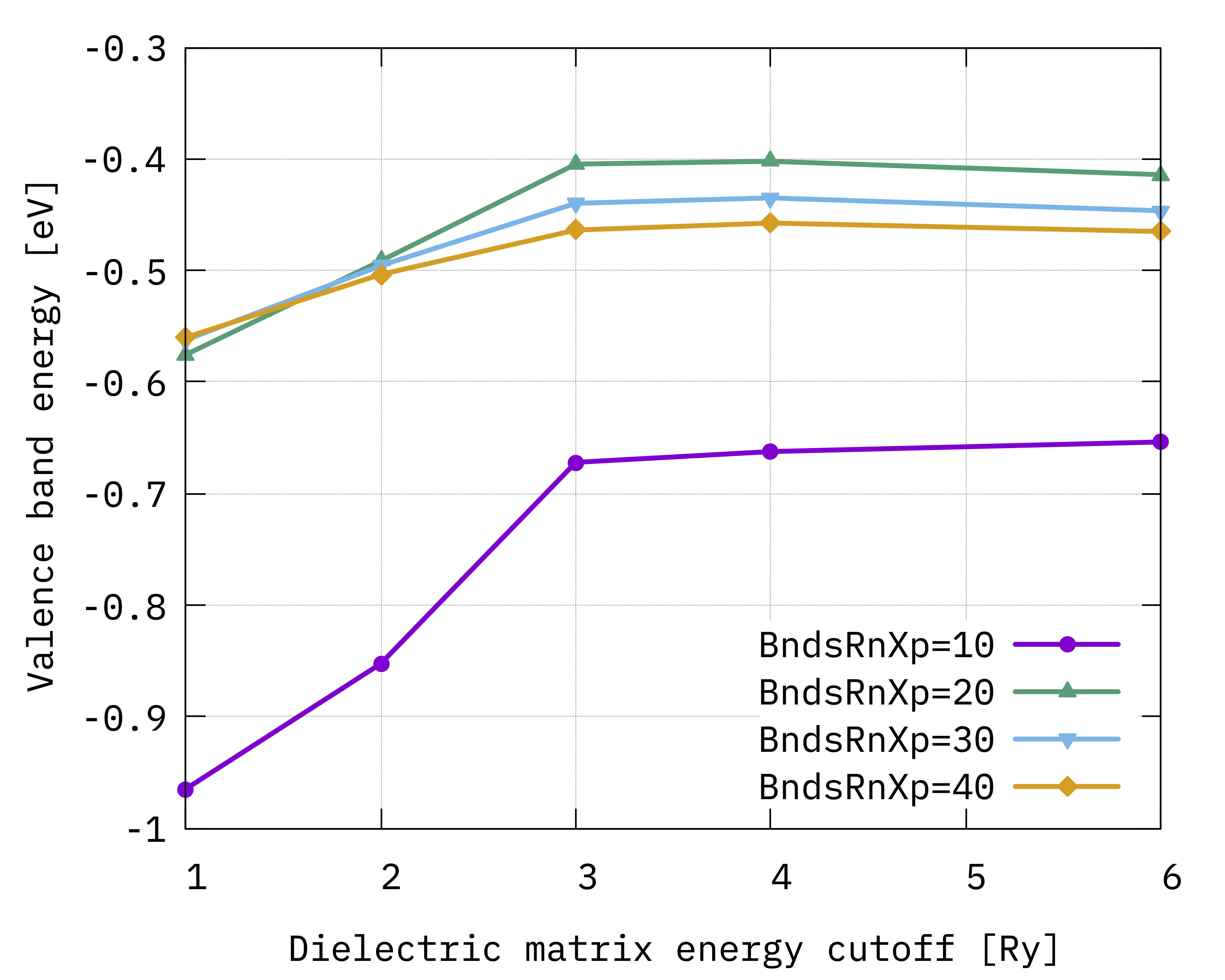
Once we have collected all the quasiparticle values, we can plot the energies of the the valence and conduction band as a function of the block size and energy cutoff.
To plot the convergence of the valence band for example type:
$ gnuplot
gnuplot> p "10b.dat" u 1:3 w lp t "BndsRnXp=10", "20b.dat" u 1:3 w lp t "BndsRnXp=20", "30b.dat" u 1:3 w lp t "BndsRnXp=30", "40b.dat" u 1:3 w lp t "BndsRnXp=40"
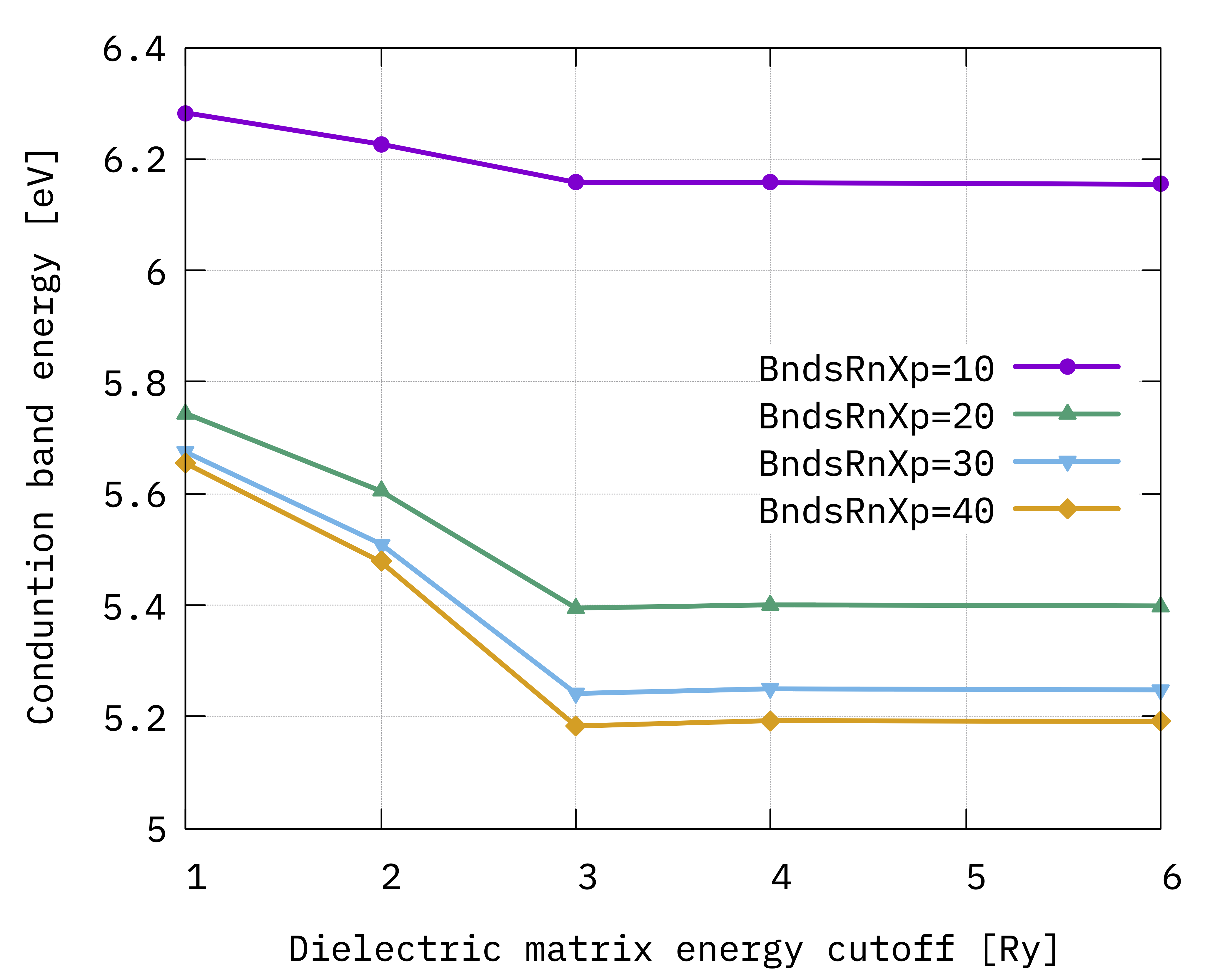
Analogously for the conduction band:
$ gnuplot
gnuplot> p "10b.dat" u 1:4 w lp t "c, BndsRnXp=10", "20b.dat" u 1:4 w lp t "c, BndsRnXp=20", "30b.dat" u 1:4 w lp t "c, BndsRnXp=30","40b.dat" u 1:4 w lp t "c, BndsRnXp=40"
You should obtain these graphs:
Attention
You may have noticed that the energy cutoff in the plots goes up to 6 Ry, despite us ranging this value between 1 and 5 Ry in input.
This happens because parse_qps.sh greps the cutoff value reported in the output file. If you check the output of the calculations run with a 5 Ry cutoff, you will see that the value actually used is 6 Ry. This is probably due to some internal rounding to include complete shells of G-vectors.
In any case, this does not affect the considerations on convergence discussed in this tutorial.
Now, we can do the same thing to plot hBN gap, using the ppa_gap.gnu gnuplot script:
ppa_gap.gnu
reset
set key c
set grid y
set grid x
set xtics nomirror
set x2tics
set autoscale xfix
set autoscale x2fix
set x2label "Cutoff Energy of eps block Ry"
set ylabel "Gap Energy eV"
set xlabel "Size of the dielectric matrix"
p "10b.dat" u 1:($4-$3)  w lp lw 2 lt -1 t "BndsRnXp=10",""  using 1:($4-$3):x2tic(2) axes x2y1 lt 7 t "" ,\
"20b.dat" u 1:($4-$3)  w lp lw 2 lt 1 t "BndsRnXp=20",""  using 1:($4-$3):x2tic(2) axes x2y1 lt 7 t "" ,\
"30b.dat" u 1:($4-$3)  w lp lw 2 lt 2 t "BndsRnXp=30",""  using 1:($4-$3):x2tic(2) axes x2y1 lt 7 t ""  ,\
"40b.dat" u 1:($4-$3)  w lp lw 2 lt 3 t "BndsRnXp=40",""  using 1:($4-$3):x2tic(2) axes x2y1 lt 7 t ""
$ gnuplot
gnuplot> load 'ppa_gap.gnu'
You should see this convergence for hBN gap:
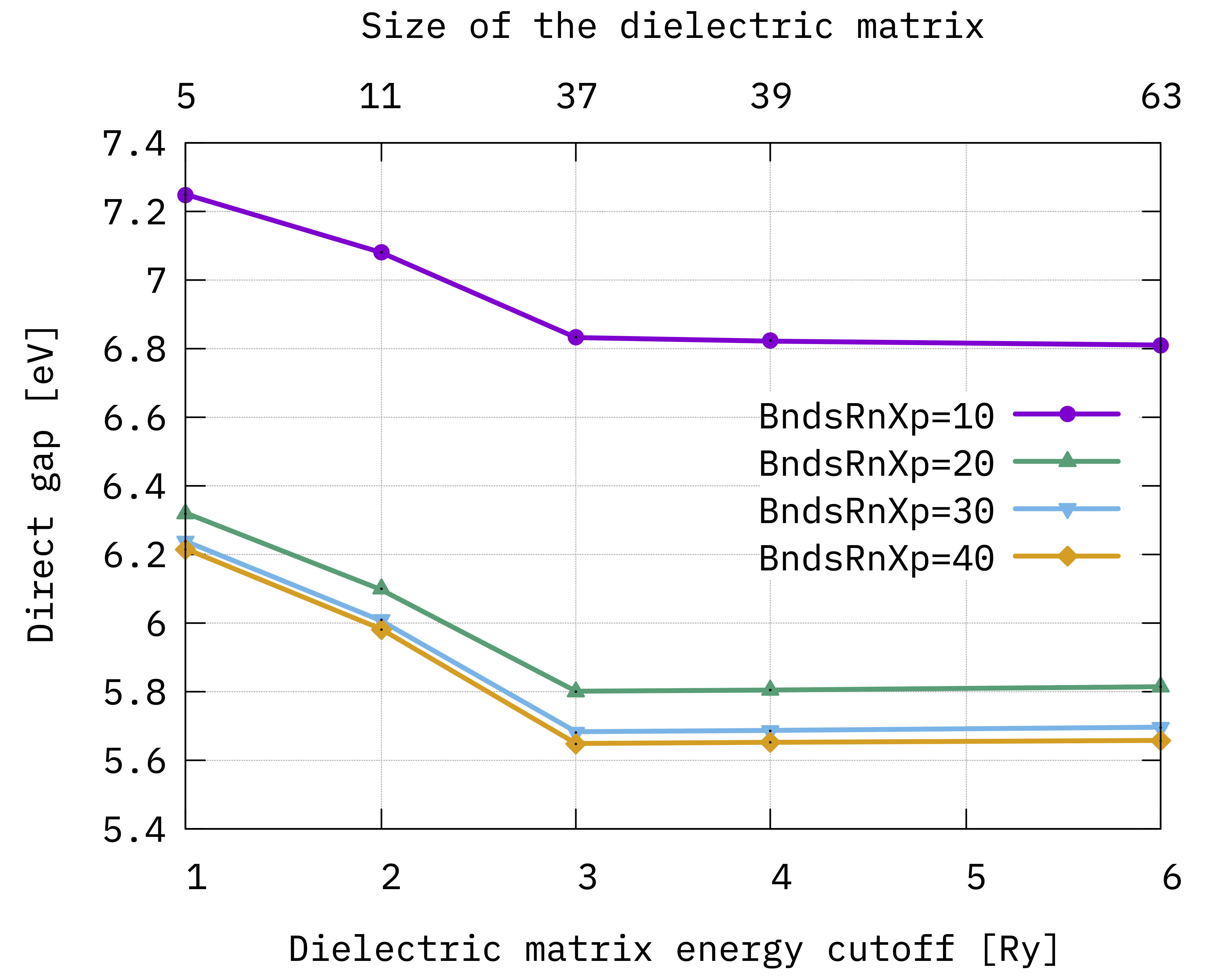
Convergence of hBN direct gap with respect to the
screening parameters BndsRnXp and NGsBlkXp.
Looking at the results we notice that:
BndsRnXpandNGsBlkXpare not totally independent on each other (see e.g. the valence quasiparticle convergence) and this is the reason why we converged them simultaneously;The gap (energy difference) converges faster than single quasiparticle state;
The convergence criteria depends on the degree of accuracy we look for, but considering the approximations behind the calculations (e.g. plasmon-pole etc.) it is not always a good idea to enforce too strict a criteria;
Even if not totally converged, for now we can consider 30 a reasonable value for the upper limit of
BndsRnXp, and 3 Ry forNGsBlkXp.
Converging the sum over states in \(\Sigma^c_{n\boldsymbol{k}}\)
Now we keep BndsRnXp and NGsBlkXp fixed to the values we decided before,
and we perform a convergence study on the sum over bands in the corration
self-energy \(\Sigma^c_{n\boldsymbol{k}}\). This is the sum over \(m\) in Eq.(3),
which is controlled by the variable GbndRnge.
To use the previously calculated screening databases (and avoid computing them
again) we can copy them from the 30b_3Ry directory to the SAVE directory.
$ cp ./30b_3Ry/ndb.pp* ./SAVE/.
In this way the screening will be read by Yambo and not calculated again, because
Yambo always looks for compatible databases in the SAVE folder.
Tip
Remember that you can achieve this also using the -J option and providing multiple
directories when running Yambo, for example
& yambo -F some_input.in -J some_new_dir,30b_3Ry
In this way the new calculation will look for available databases first in some_new_dir
and then in 30b_3Ry, where it will find the necessary data. New databases will be
printed in some_new_dir.
Caution
Always be careful when you move databases in the SAVE folder because
they could interfere with future calculations.
Important
Remember that to use the saved databases, we must be sure to have exactly the same parameters in our input files.
Edit gw_ppa_30b_3Ry.in and modify GbndRnge in to order to have a number
of bands in the range from 10 to 80 inside different files named gw_ppa_Gbnd10.in,
gw_ppa_Gbnd20.in and so on.
As before, you can use the generate_and_run_inputs_2.sh bash script below to generate the
required input files and run the calculations.
generate_and_run_inputs_2.sh
#!/bin/bash
#
# Gbnd convergence input files
#
bands='10 20 30 40 50 60 70 80'
for i in ${bands}
do
  sed  -e "s/1 | 40/1 | $i/g"  gw_ppa_30b_3Ry.in  >  gw_ppa_Gbnd$i'.in'
  yambo -F gw_ppa_Gbnd$i'.in' -J Gbnd$i
done
Remember to make it executable with
chmod +x generate_and_run_inputs_2.sh.
Next, launch all the calculations
$ ./generate_and_run_inputs_2.sh
We can take a look to the quasiparticle energies for the valence band:
$ grep "7 * 8" o-Gbnd* | awk '{print $4+$5}'
and for the conduction band:
$ grep "7 * 9" o-Gbnd* | awk '{print $4+$5}'
Collect the results in a text file Gbnd_conv.dat containing:
the number of bands included in the sum (i.e.
GbndRnge);the valence quasiparticle energy;
the conduction quasiparticle energy.
As before, we plot the valence and conduction quasiparticle levels separately as well as the gap as a function of the number of bands used in the sum over states:
$ gnuplot
gnuplot> p "Gbnd_conv.dat" u 1:2 w lp lt 7  t "Valence"
gnuplot> p "Gbnd_conv.dat" u 1:3 w lp lt 7  t "Conduction"
gnuplot> p "Gbnd_conv.dat" u 1:($3-$2) w lp lt 7  t "Gap"
Compare your results with the figures reported below.
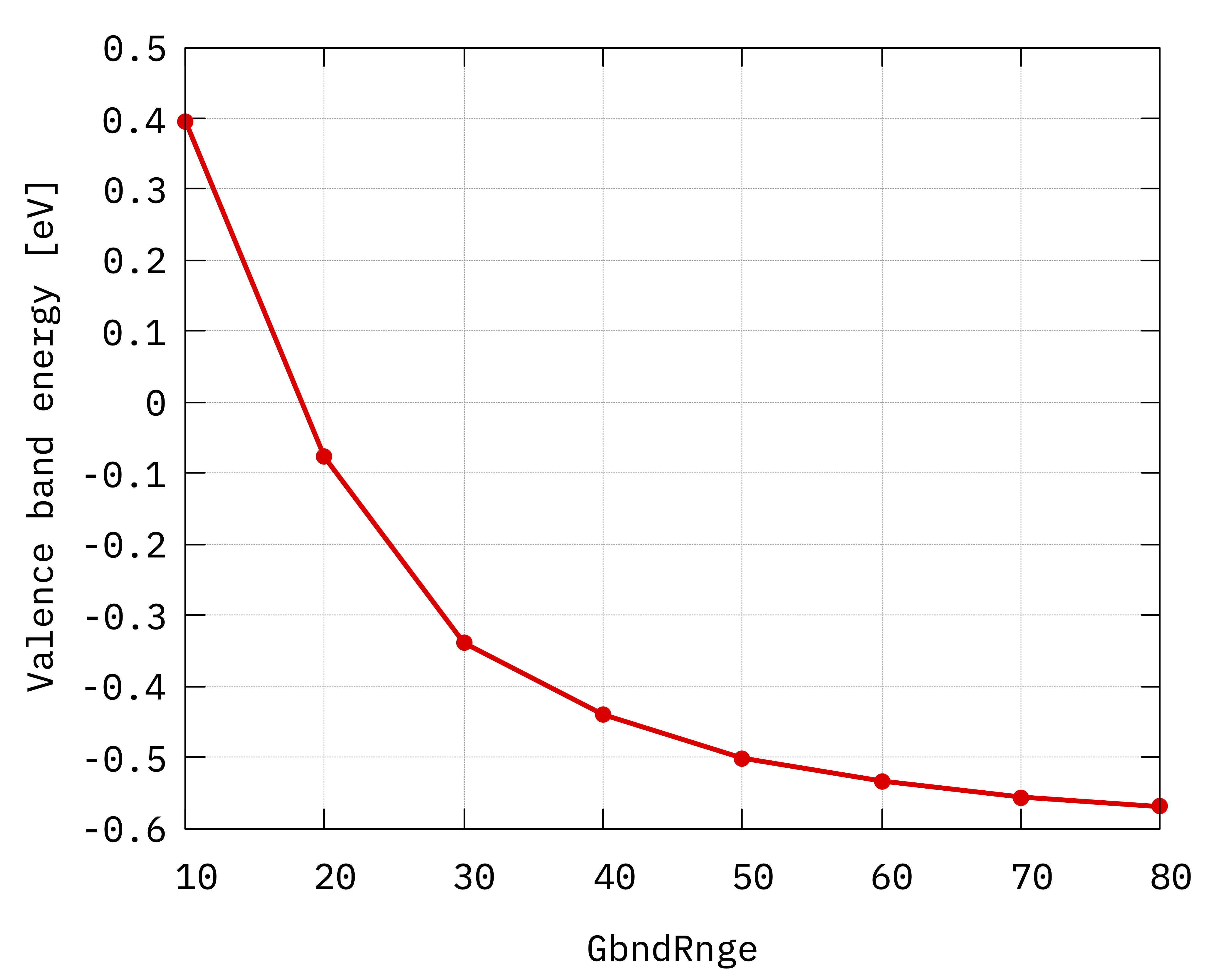
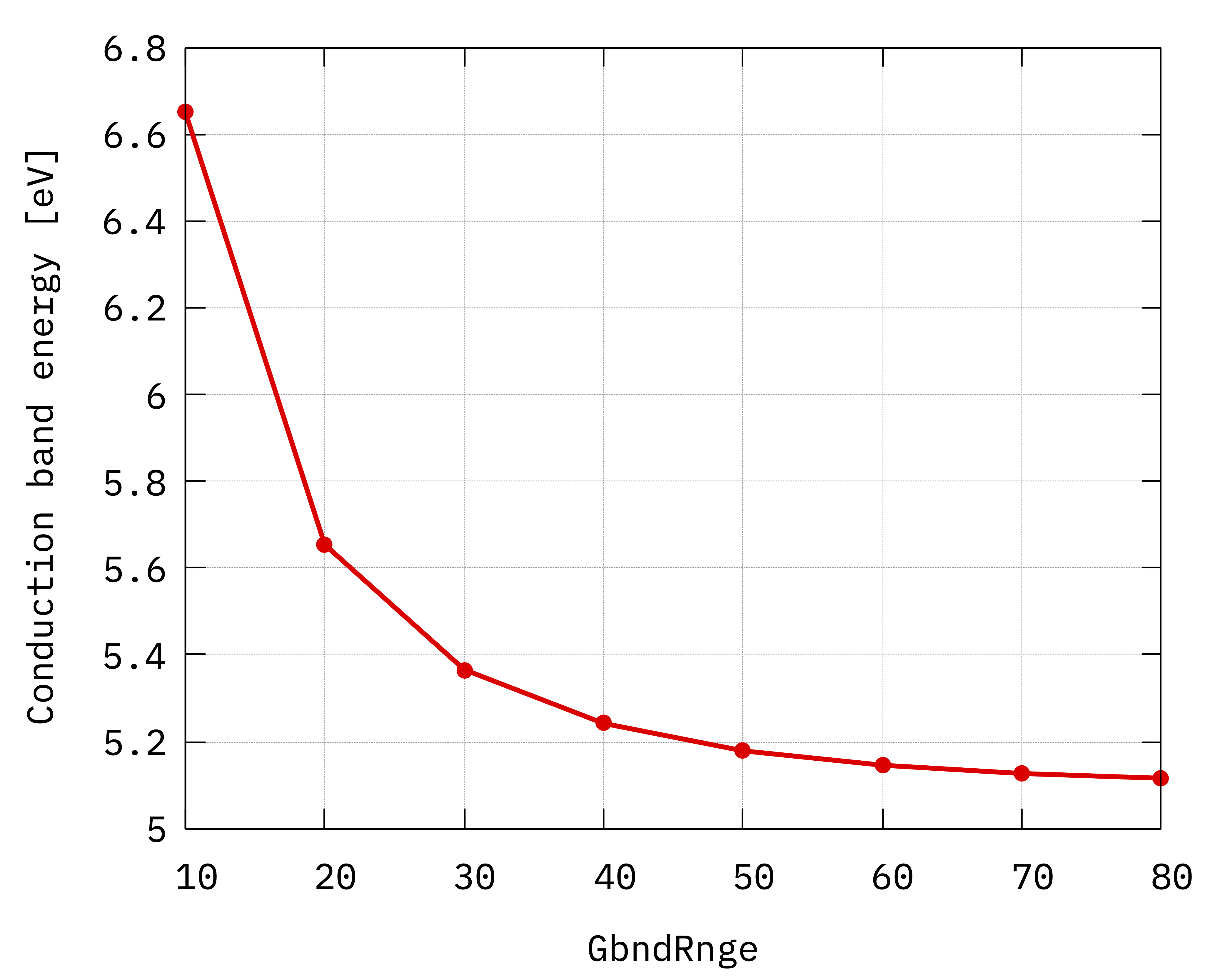
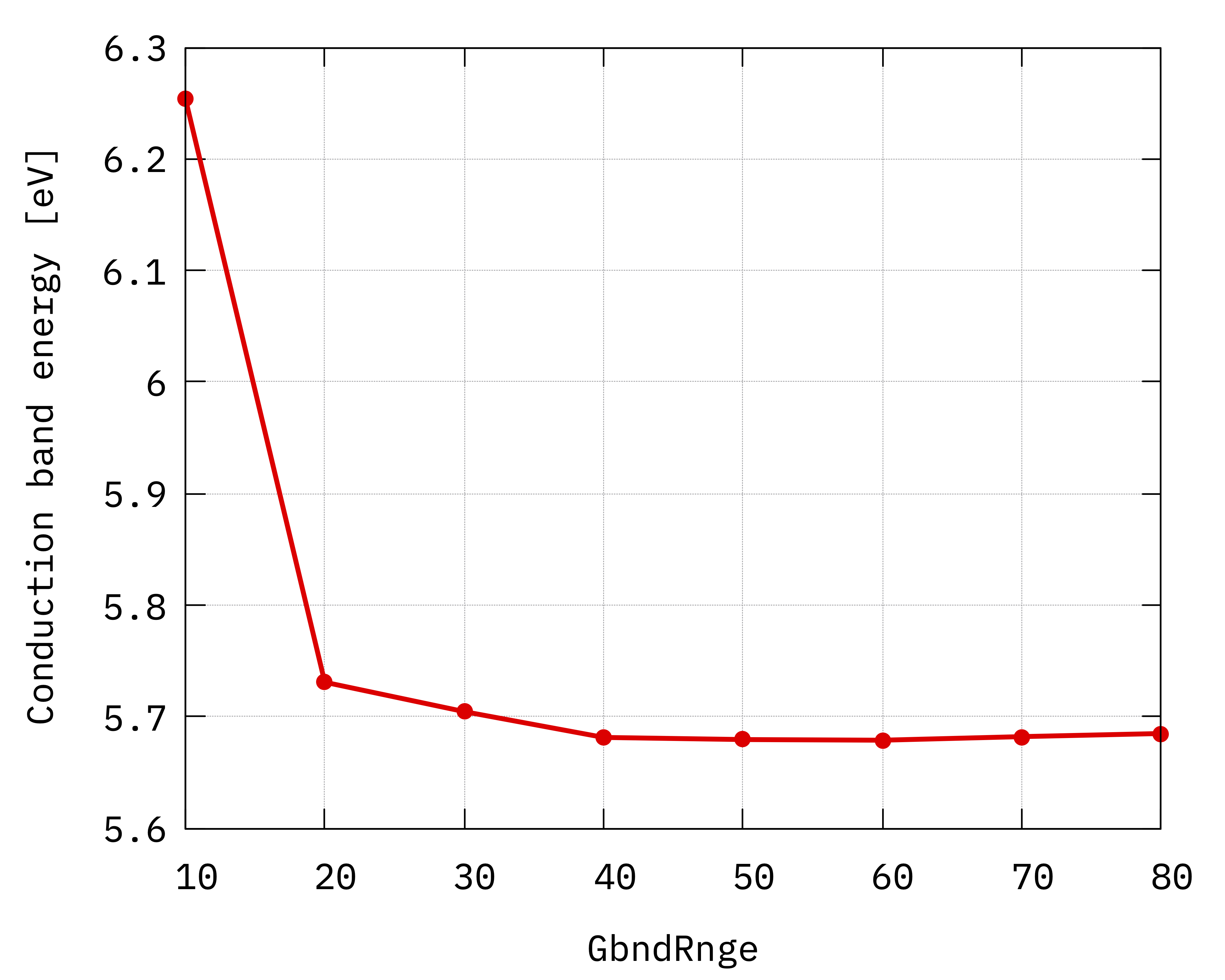
Convergence of hBN direct gap with respect to the
sum over states parameter GbndRnge.
Inspecting the plots we can notice that:
The convergence with respect to
GbndRangeis rather slow and many bands are needed to get converged results.As observed previously, the gap (energy difference) converges faster than the energies of single quasiparticle states.
Alternative approach to convergence (optional)
In this example we keep the same value for both BndsRnXm and GbndRnge, so “number of bands” refers to both of them.
We can follow the scheme proposed in this article[1] for converging the dielectric matrix energy cutoff (i.e. NGsBlkXm) and the number of bands: choose a value for one of the two and converge the other; when convergence with respect to this one is reached, keep it fixed and start converging the other one; continue until the QP energies are converged within the threshold that you want.
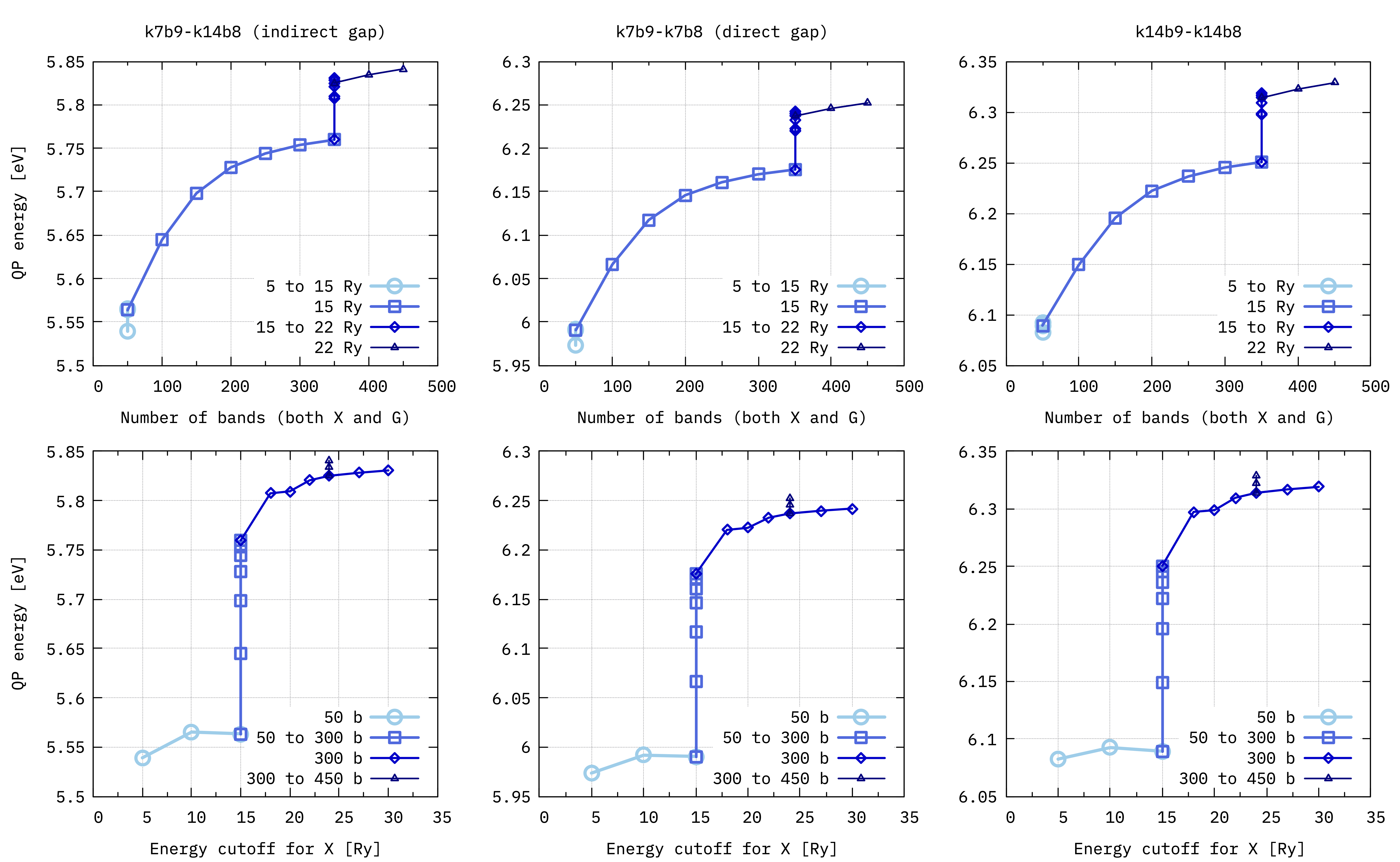
Convergence of hBN QP gaps with respect to NGsBlkXp and the number of bands (BndsRnXm and GbndRnge). The top and bottom rows show the same values plotted vs number of bands (top) and dielectric matrix cutoff (bottom). The plots in the middle column show the direct gap located at \(\boldsymbol{k}\) point n. 7 between bands \(n=8\) and \(n=9\).
Note
The parameters used to produce the plots shown here are very large compared to the ones used in the other sections of this tutorial. If you want to reproduce these results, we suggest to run the calculations in parallel.
k points convergence (optional)
The last important convergence test deals with the accuracy of the integral over the Brillouin zone in the expression of the correlation self-energy (Eq. (3)) and of the dielectric function ( through Eq. (9)). Do not forget that in a full GW calculation this integral we are referring to appears also in the exchange part of the self-energy (see Hartree-Fock tutorial.
To test the convergence with respecto to the k-point sampling, you should:
Perform a new non-scf calculation with a denser k-grid;
Convert wave functions and electronic structure to Yambo databases in a different directory;
Initialize the new Yambo databases;
Redo the steps explained in this tutorial for each k-grid.
Note that the use of denser k-point grids increases quite significantly the computational load of the calculation, and this usually cannot be avoided. GW calculations in general require much denser grids than DFT calculations to converge.
Important
In good part, the slower convergence in the k-grid size with respect to DFT is due to \(\epsilon^{-1}_{\mathbf{G},\mathbf{G'}}\), which is the quantity most sensible on the k-points sampling within a GW calculation.
There are however techniques available in Yambo that accelerate the convergence with respect to the k-grid which are discussed in specific tutorials.
Tip
Below are some useful general recommendations:
To reduce the computational cost, first test the convergence of the parameters discussed above (
BndsRnXp,NGsBlkXp, andGbndRange) using a coarse k-grid;Next, perform the convergence study with respect to the k points while keeping the other parameters fixed at reasonable, but not fully converged values;
Once determined satisfactory values for all parameters, perform a final check with fully converged parameters to confirm your choices.
Full GW band structure
Once we have determined the values of the critical parameters we can proceed with computing the quasiparticle corrections across all of the Brillouin zone so we can eventually visualize the entire band structure along a path connecting high symmetry points.
To do this we start by calculating the QP corrections in the plasmon-pole approximation for all the k points and for a number of bands around the gap.
You can use a previous input file or generate a new one:
$ yambo -F gw_ppa_all_Bz.in -x -p p -g n
Set the parameters found in the previous convergence tests:
EXXRLvcs=  40              Ry      # [XX] Exchange    RL components
% BndsRnXp
  1 | 30 |                         # [Xp] Polarization function bands
%
NGsBlkXp=  3              Ry       # [Xp] Response block size
% LongDrXp
 1.000000 | 1.000000 | 1.000000 |  # [Xp] [cc] Electric Field
%
% GbndRnge
   1 | 40 |                        # [GW] G[W] bands range
%
%QPkrange                          # [GW] QP generalized Kpoint/Band indices
1|14|6|11|
%
Note that we already have the screening databases corresponding to these parameters, so you can use them and avoid computing them again.
Attention
Remove any ndb.pp* databases you may have in the SAVE folder before continuing!
$ rm SAVE/ndb.pp*
You can either copy ndb.pp* databases from 30b_3Ry in a new folder named all_Bz and then
run yambo -F gw_ppa_all_Bz.in -J all_Bz or use the -J option to avoid duplicating the files:
$ yambo -F gw_ppa_all_Bz.in -J all_Bz,30b_3Ry
l-all_Bz_HF_and_locXC_gw0_dyson_em1d_ppa_el_el_corr
  __ __  ____ ___ ___ ____   ___
 |  |  |/    |   |   |    \ /   \
 |  |  |  o  | _   _ |  o  )     |
 |  ~  |     |  \_/  |     |  O  |
 |___, |  _  |   |   |  O  |     |
 |     |  |  |   |   |     |     |
 |____/|__|__|___|___|_____|\___/


 <---> [01] MPI/OPENMP structure, Files & I/O Directories
 <---> MPI Cores-Threads   : 1(CPU)-48(threads)
 <---> [02] CORE Variables Setup
 <---> [02.01] Unit cells
 <---> [02.02] Symmetries
 <---> [02.03] Reciprocal space
 <---> [02.04] K-grid lattice
 <---> Grid dimensions      :   6   6   2
 <---> [02.05] Energies & Occupations
 <---> [03] Transferred momenta grid and indexing
 <---> [WARNING] [Xp] User bands 1-30 break level degeneracy
 <---> [04] Dipoles
 <---> [04.01] Setup: observables and procedures
 <---> [05] Dynamic Dielectric Matrix (PPA)
 <---> Loading the dielectric function |########################################| [100%] --(E) --(X)
 <---> [06] Local Exchange-Correlation + Non-Local Fock
 <---> [FFT-HF/Rho] Mesh size:   18   18   44
 <02s> EXS |########################################| [100%] --(E) --(X)
 <02s> [xc] Functional : Slater exchange(X)+Perdew & Zunger(C)
 <02s> [xc] LIBXC used to calculate xc functional
 <04s> [06.01] Hartree-Fock occupations report
 <04s> [07] Dyson equation: Newton solver
 <04s> [07.01] G0W0 (W PPA)
 <04s> [FFT-GW] Mesh size:  12  12  27
 <02m-55s> G0W0 (W PPA) |########################################| [100%] 02m-51s(E) 02m-51s(X)
 <02m-56s> [07.02] QP properties and I/O
 <02m-56s> [08] Timing Overview
 <02m-56s> [09] Memory Overview
 <02m-56s> [10] Game Over & Game summary
If we look into the output we see that now we have quasiparticle corrections for all kpoints and bands we asked for:
$ grep -A9 '#    K-point' o-all_Bz.qp
#    K-point            Band               Eo [eV]            E-Eo [eV]          Sc|Eo [eV]
#
        1                   6                -1.299712          -0.198659           3.812934
        1                   7                -1.296430          -0.221065           3.812979
        1                   8                -1.296420          -0.222893           3.810808
        1                   9                 4.832399           0.932613          -3.704120
        1                  10                 10.76416           2.081852          -4.412297
        1                  11                 11.36167           2.462667          -3.935066
        2                   6                -1.335548          -0.202082           3.819093
        2                   7                -1.335520          -0.200409           3.821062
By plotting some of the columns from o-all_Bz.qp it is possible to discuss some physical properties
of the hBN QPs.
Using columns 3 and 3+4, ie plotting the GW energies with respect to the DFT energies we can deduce
the band gap renormalization and the stretching of the conduction/valence bands:
$ gnuplot
gnuplot> p "o-all_Bz.qp" u 3:($3+$4) w p t "E_Q_P vs E_0"
This produces the following plot:
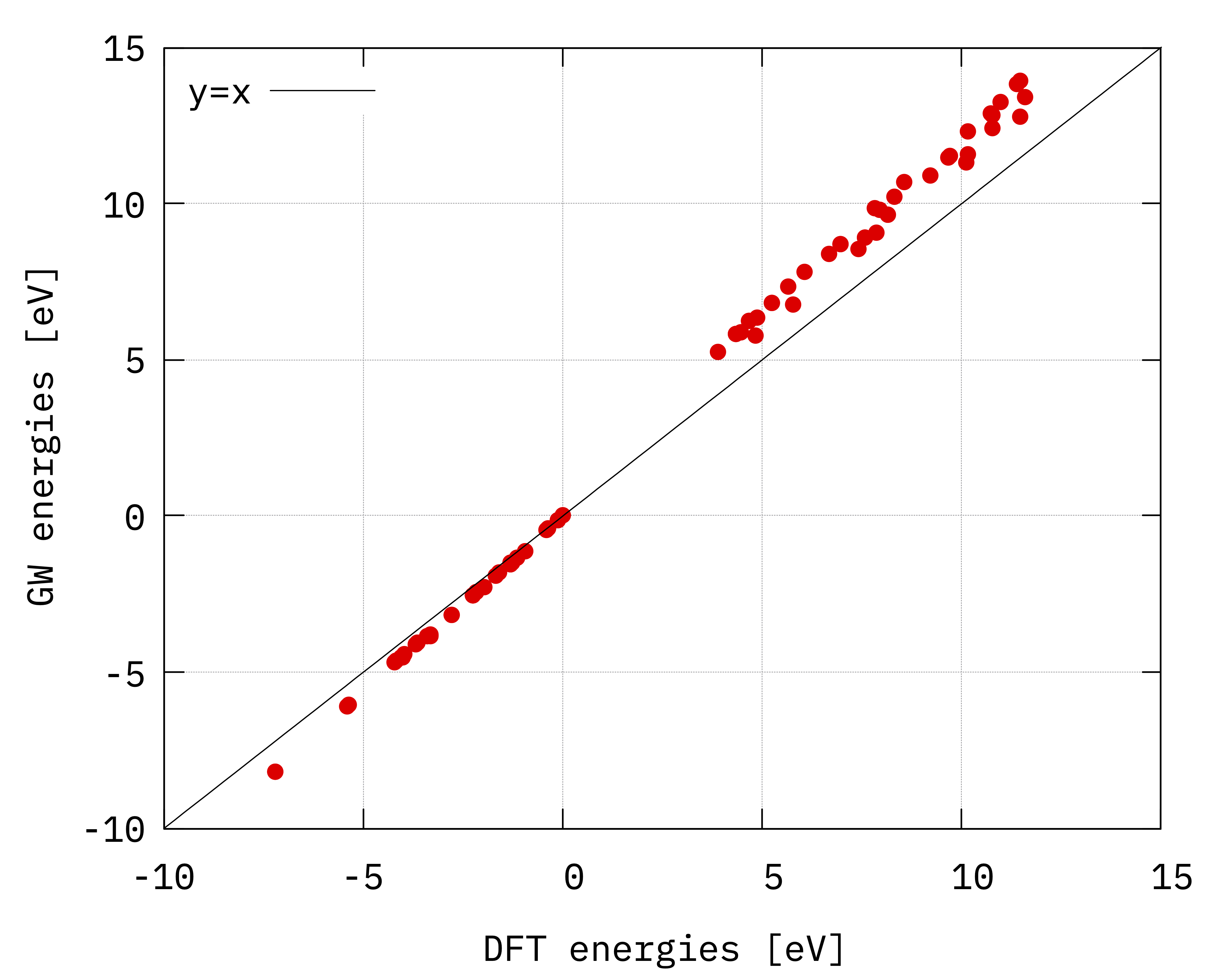
Plot of quasiparticle energies vs DFT energies. The black lines (\(y=x\)) highlights the different stretching (slope) of the valence and conduction bands.
Essentially we can see that the effect of the GW self-energy is the opening of the gap (notice that the gap along the horizontal/DFT axis is less than 5 eV while it’s bigger than 5 eV along the vertical/quasiparticle axis) and a linear stretching of the conduction/valence bands that can be estimated by performing a linear fit of the positive and negative energies (remember that the zero is set at top of the valence band).
Tip
Yambopy provides a tool to do this fit and thus provide the parameters for the scissor operator. This can be used to extrapolate the GW energies directly from the DFT ones without doing the explicit calculation.
In order to calculate the band structure, however, we need to interpolate the values we have
calculated above on a given path.
In Yambo you can do the interpolation using the executable ypp (Yambo Post Processing).
Note
You can also use Yambopy.
From ypp -h you can see that the right option to do the interpolation of the bands is
-electrons bands or, in short,
$ ypp -s b -F ypp_bands.in
Then set these input variables as follows:
INTERP_mode= "BOLTZ"
OutputAlat= 4.716000
% BANDS_bands
   6 | 11 |
%
BANDS_steps= 30
%BANDS_kpts
 0.33300 |-.66667 |0.00000 |
 0.00000 |0.00000 |0.00000 |
 0.50000 |-.50000 |0.00000 |
 0.33300 |-.66667 |0.00000 |
 0.33300 |-.66667 |0.50000 |
 0.00000 |0.00000 |0.50000 |
 0.50000 |-.50000 |0.50000 |
%
which means we assign 30 points in each segment, we ask to interpolate 3 occupied (6 to 8) and 3 empty (9 to 11) bands and we assign the following path passing through the high symmetry points: \(K\) \(\Gamma\) \(M\) \(K\) \(H\) \(A\) \(L\).
We can now launch ypp:
$ ypp -F ypp_bands.in
This produces the output file o.bands_interpolated:
$ grep -A5 '#     |k| (a.u.)' o.bands_interpolated
#     |k| (a.u.)         b6                 b7                 b8                 b9                 b10                b11               k_x (rlu)          k_y (rlu)          k_z (rlu)
#
       0.00000000        -7.22092473       -0.134022118       -0.133954835         4.67690928         4.67694609         10.0890450        0.333000000       -0.666670000         0.00000000
      0.296070964E-1     -7.18831883       -0.172395273       -0.127192594         4.66612681         4.70859775         10.1194847        0.321900000       -0.644447667         0.00000000
      0.592141929E-1     -7.09275720       -0.288027880       -0.113852112         4.64448157         4.80302722         10.2015775        0.310800000       -0.622225333         0.00000000
      0.888212893E-1     -6.94016497       -0.476628552       -0.108512380         4.63275992         4.95459111         10.3109048        0.299700000       -0.600003000         0.00000000
However this performs the interpolation on the bands. You can realize this by
quickly plotting the bands with gnuplot
(p "o.bands_interpolated" u 0:2 w l, "" u 0:3 w l, ...)
To get the GW bands we need to tell ypp the path to the ndb.QP database.
This is done by adding the following line anywhere in the ypp_bands.in input file:
GfnQPdb= "E < ./all_Bz/ndb.QP"
Run ypp -F ypp_bands.in as before. The new bands will be printed in o.bands_interpolated_01.
Note
Now a new section External/Internal QP corrections appears in the report file
r_electrons_bnds_01. You may also notice that a new ndb.QP_interpolated
database is written in the SAVE folder.
You can now compare the DFT and GW bands by plotting them (using the bands.gnu gnuplot script
below if you want).
bands.gnu
set xtics ("K" 0, "{/Symbol G}" 30, "M" 56, "K" 71, "H" 80, "A" 110, "L" 136)

set ylabel "Energy [eV]"

p   "o.bands_interpolated" u 0:2 w l lt -1 t "DFT"
rep "o.bands_interpolated" u 0:3 w l lt -1 t ""
rep "o.bands_interpolated" u 0:4 w l lt -1 t ""
rep "o.bands_interpolated" u 0:5 w l lt -1 t ""
rep "o.bands_interpolated" u 0:6 w l lt -1 t ""
rep "o.bands_interpolated" u 0:7 w l lt -1 t ""

rep "o.bands_interpolated_01" u 0:2 w l lt 7 t "GW"
rep "o.bands_interpolated_01" u 0:3 w l lt 7 t ""
rep "o.bands_interpolated_01" u 0:4 w l lt 7 t ""
rep "o.bands_interpolated_01" u 0:5 w l lt 7 t ""
rep "o.bands_interpolated_01" u 0:6 w l lt 7 t ""
rep "o.bands_interpolated_01" u 0:7 w l lt 7 t ""
Save this in a file named bands.gnu and then load it in gnuplot to
plot the bands:
$ gnuplot
gnuplot> load 'bands.gnu'
Tip
ypp writes the high symmetry points at the end of the corresponding lines
in the output file.
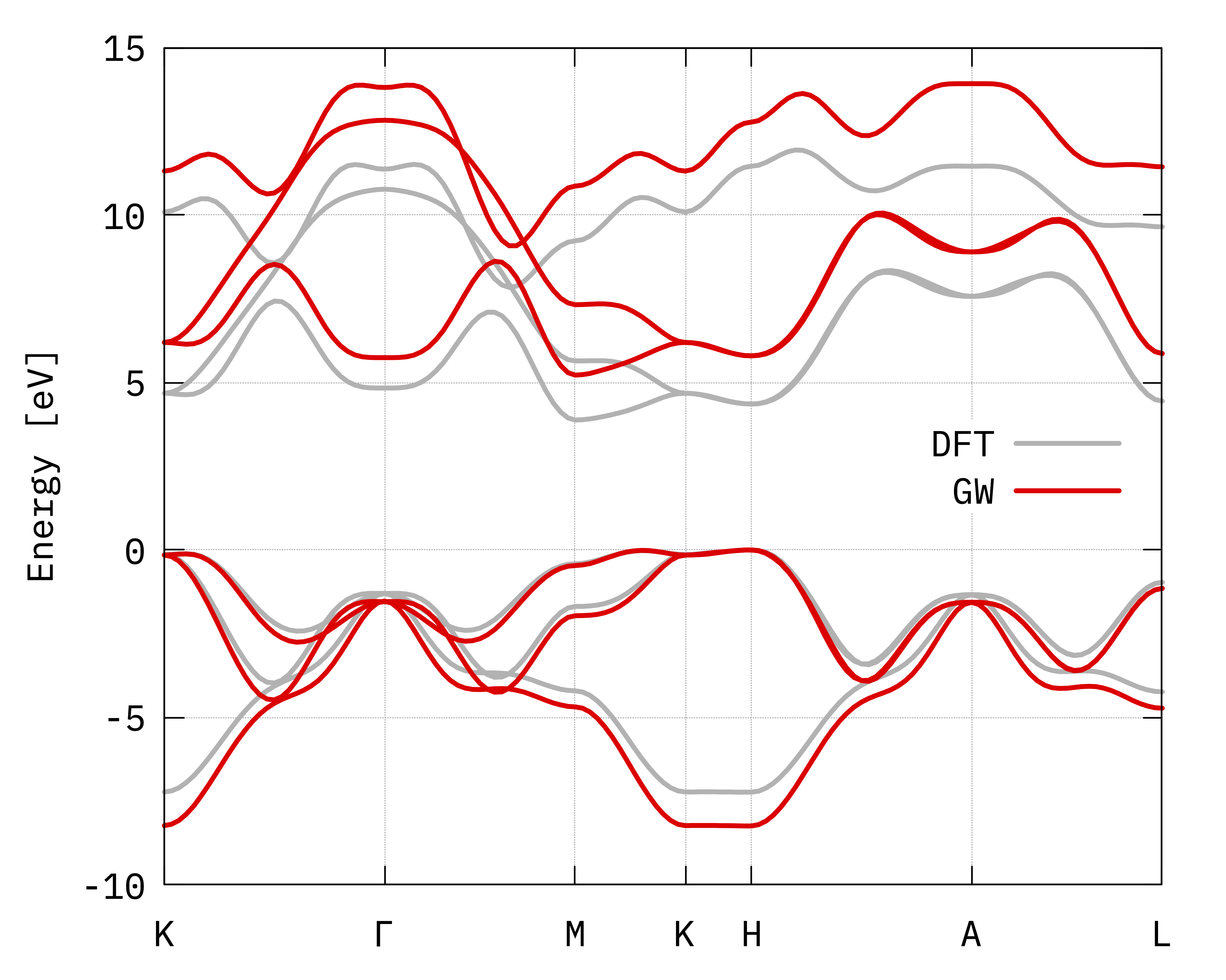
GW bands of bulk hBN compared to the DFT ones.
Some final considerations:
As expected the effect of the GW correction is to open the gap;
Comparing the obtained band structure with the one found in the literature (see e.g. this article[2]) we found a very nice qualitative agreement. Quantitatively we find a smaller gap (about 5.2 eV for the indirect gap and about 5.7 eV for the direct gap) than the one reported in Arnaud et al. (5.95 eV for the indirect gap and a minimum direct band gap of 6.47 eV). Other values are also reported in the literature depending on the pseudopotentials used, the starting functional and self-consistency accuracy.
Finally, remember that the convergence with respect to k points is very important in order to get accurate results.