GW on MoS2: parallelization schemes
In this tutorial we will focus on the parallelization strategies available in Yambo for a GW calculation. We will use 2D MoS2 as an example system.
Requirements
SAVEfolder of 2D MoS2: download and extractMoS2_HPC_tutorial.tar.gzfrom the Tutorial files page.yamboexecutableyppexecutable (optional)pythonin order to use some of the provided scriptsgnuplot(optional) for plotting some of the results
It is assumed that you are familiar with the concepts related to the SAVE folder and handling files with Yambo.
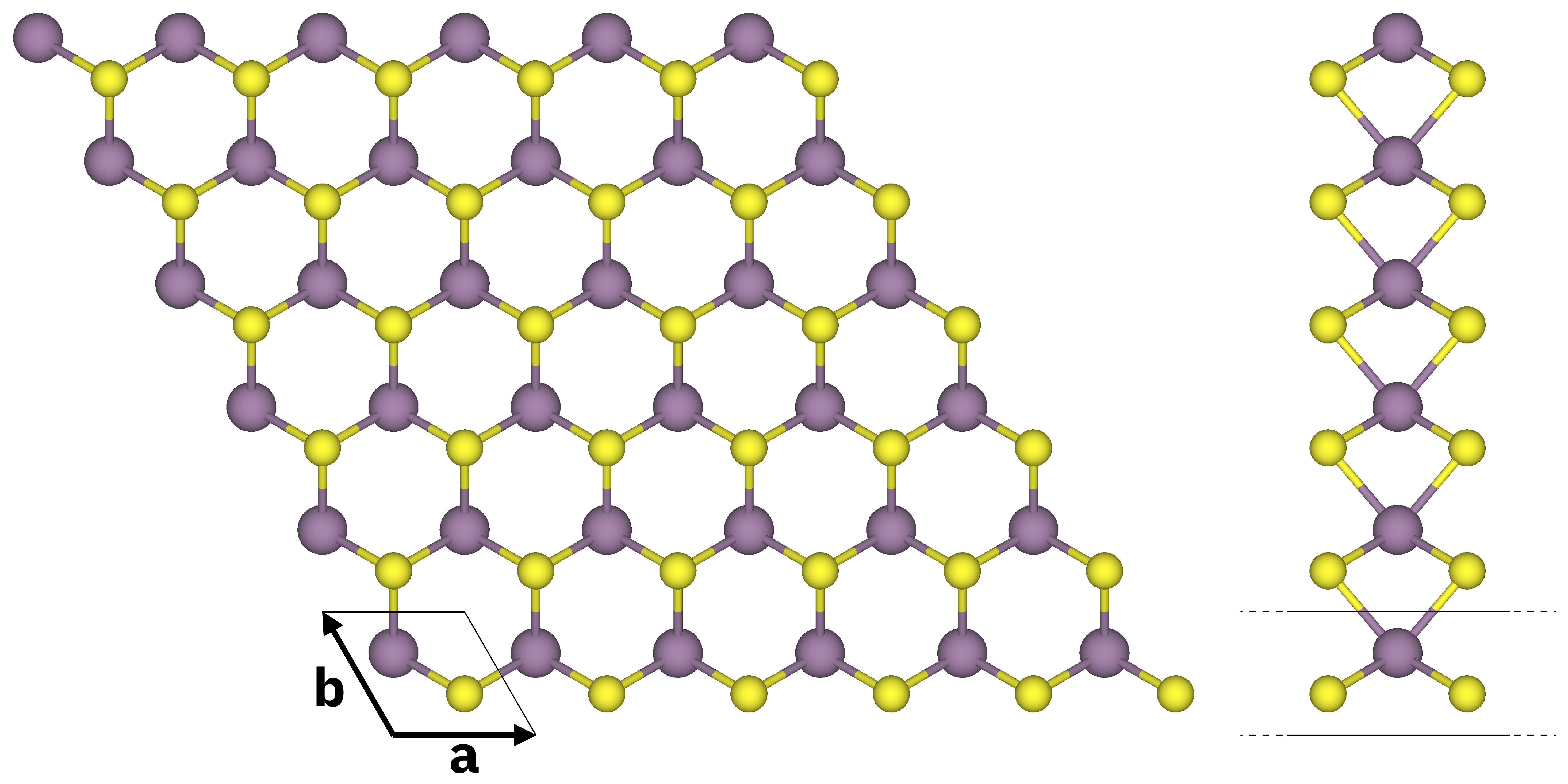
Atomic structure of monolayer MoS2 (top and side views). S atoms in yellow, Mo atoms in purple. The solid black lines mark the unit cell.
In order to appraise the speedup gained by running Yambo in parallel, the calculations in this tutorial are quite hefty and they are meant to be run on a HPC machine.
Important
You may need to adjust the parallelization scheme to the specifics of the machine where you are running the tutorial. If you find that the calculations are too slow, try using more resources (if you can) or decreasing the values of relevant parameters. If you are at a school, check the school main page for indications.
Quick overview of parallelization in Yambo
In general, we have in mind two different possibilities: running Yambo on CPUs or on GPUs.
In the examples below we consider the parallelization scheme for the calculation of dipoles (the coupling strengths of electrons with optical light), one of the most common runlevels in Yambo. The calculation of dipoles can be parallelized over k points, conduction bands and valence bands, so in the input file we set
DIP_ROLEs= "k c v" # [PARALLEL] CPUs roles (k,c,v)
and decide how to distribute the calculation using the corresponding DIP_CPU variable, like this:
DIP_CPU= "2 4 1" # [PARALLEL] CPUs for each role
Some parts of Yambo use OPENMP parallelization, so there are also variables that control the number of OPENMP threads.
In the case of dipoles, the variable is DIP_THREADS:
DIP_Threads=2 # [OPENMP/X] Number of threads for dipoles
Note
The *_Threads input variables overwrite the OMP_NUM_THREADS environment variable, unless they are set =0 (in which case Yambo uses the value of OMP_NUM_THREADS).
To keep the discussion as simple as possible in the following examples we do not consider hyper-threading (i.e. we just consider a CPU to be made of a certain number of cores).
Running Yambo on CPU:
In the case of a pure MPI run, one can assign up to one MPI task for each physical core.
However typically we have both MPI and OPENMP. In this hybrid case the best performance is often obtained assigning 2, 4, 8 or even more OPENMP threads and setting the number of MPI tasks so that the product of these two values equals the total number of cores.
Example
Let’s say you are running a calculation on 2 nodes of a cluster where each node has a total of 32 CPU cores. Then you can set
DIP_ROLEs= "k c v"
DIP_CPU= "4 4 2"
DIP_THREADS=2
or
DIP_ROLEs= "k c v"
DIP_CPU= "4 4 4"
DIP_THREADS=1
or even
DIP_ROLEs= "k c v"
DIP_CPU= "2 4 1"
DIP_THREADS=8
Calculations on CPUs run much slower compared to GPUs, so typically a large number of nodes (and consequently MPI tasks) is required.
Note
CPU nodes with a large number of cores (64 and above) are becoming more common. In this cases it is strongly recommended to avoid using only MPI: better performances are obtained balancing the number of MPI tasks and OPENMP threads.
Running Yambo on GPU:
In the case of GPUs, you must assign one MPI task per GPU.
Example
Considering a case where you run a calculation on 2 nodes where each node has 4 GPUs and one 16-core CPU, you can set
DIP_ROLEs= "k c v"
DIP_CPU= "2 4 1"
DIP_THREADS=4
or
DIP_ROLEs= "k c v"
DIP_CPU= "2 2 2"
DIP_THREADS=4
or even
DIP_ROLEs= "k c v"
DIP_CPU= "8 1 1"
DIP_THREADS=4
Notice that in this case the number of OPENMP threads is fixed by the architecture of the node: since we must assign one MPI task per GPU, we choose the number of OPENMP threads so that its product with the number of MPI tasks per node gives exactly the total number of threads of the CPU installed in the node (16 in this example).
We are now ready to proceed with the tutorial, keeping in mind the following:
Important
The best parallelization scheme is determined by the hardware architecture as well as by the parameters of the system you are studying. The best practice is always to test different parallelization schemes, especially when dealing with very large calculations.
Many-body corrections to the DFT energy levels
We want to describe the electronic energy levels using a better description of electron-electron interactions than DFT is capable of. To do so we essentially need to solve the non-linear quasiparticle equation involving the GW self-energy \(\Sigma\):
A more detailed discussion of the underlying theory and its practical implementation is provided at the beginning of this tutorial.
In what follows, we deliberately omit any discussion of convergence with respect to the relevant parameters. As noted earlier, these parameters may need to be adjusted to match the computational resources available on your machine. Consequently, the final results presented here should be regarded as illustrative rather than quantitatively accurate.
See also
You may find very useful to check these cheatsheets, where you can find the quantities calculated by Yambo and the input file variables related to them, included those controlling the parallelization.
Set up a Yambo calculation
The SAVE folder
As always, the very first step in a Yambo calculation is to generate the SAVE folder converting the data from the DFT calculation and initialize it right after that.
The SAVE folders we will use in this tutorial are already initialized.
Remember that you can verify this by looking for the presence of the databases ndb.gops and ndb.kindx in the SAVE folder.
Go to the 01_GW_first_run and check that the SAVE folder is already initialized:
$ cd MoS2_HPC_tutorial/01_GW_first_run/
$ ls -l SAVE/ndb.*
SAVE/ndb.gops
SAVE/ndb.kindx
Yambo input file
Let’s now generate the input file we will be using for our first GW calculation.
This can be done by the yambo executable via command-line instructions:
$ yambo -gw0 p -g n -r -V par -F gw.in
Tip
Type yambo -h for the full list of options.
Attention
You may need to run this command in an interactive session after loading the environment (modules, libraries and so on) required by your specific compilation of Yambo.
With these options we generate an input file where we use the plasmon pole approximation for the dynamical screening (-gw0 p), solve the quasiparticle equation with the Newton method (-g n), and add a truncation of the Coulomb potential which is useful for 2D systems (-r).
In addition, we want to set up explicitly the parameters for parallel runs (-V par).
You can now inspect the input file gw.in and try to familiarize with some of the parameters.
The input will come with default values for many parameters that we might need to change.
We recall them quickly here below.
Runlevels
gw0            # [R] GW approximation
ppa            # [R][Xp] Plasmon Pole Approximation for the Screened Interaction
el_el_corr     # [R] Electron-Electron Correlation
dyson          # [R] Dyson Equation solver
rim_cut        # [R] Coulomb potential
HF_and_locXC   # [R] Hartree-Fock
em1d           # [R][X] Dynamically Screened Interaction
These flags tell Yambo which parts of the code should be executed. Each runlevel enables its own set of input variables. Here we have:
gw0: Yambo learns that it has to run a GW calculation (enables [GW] variables).ppa: tells Yambo that the dynamical screening should be computed in the plasmon pole approximation ([Xp] variables).el_el_corr: in the case of a GW calculation this is equivalent togw0dyson: Yambo will solve the Dyson-like quasiparticle equation.rim_cut: Coulomb potential random integration method and cutoff (enables [RIM] and [CUT] variables).HF_and_locXC: calculation of exchange part of the self-energy \(\Sigma^x\) (i.e., Hartree-Fock approximation).em1d: enables the calculation of the dynamical screening of the electrons, i.e. the dielectric matrix ([X] variables). In this way Yambo can go beyond Hartree-Fock and compute \(\Sigma^c\).
Exchange self-energy
EXXRLvcs=  37965  RL   # [XX] Exchange    RL components
VXCRLvcs=  37965  RL   # [XC] XCpotential RL components
EXXRLvcscontrols the number of Reciprocal Lattice vectors (i.e., G-vectors) used to build the exchange self-energy.VXCRLvcsdoes the same for the exchange-correlation potential reconstructed from DFT.
For a more in-depth discussion on this part of the calculation see the Hartree-Fock tutorial.
Response function
Chimod= "HARTREE"                  # [X] IP/Hartree/ALDA/LRC/PF/BSfxc
% BndsRnXp
   1 | 300 |                       # [Xp] Polarization function bands
%
NGsBlkXp= 1                RL      # [Xp] Response block size
% LongDrXp
 1.000000 | 0.000000 | 0.000000 |  # [Xp] [cc] Electric Field
%
PPAPntXp= 27.21138         eV      # [Xp] PPA imaginary energy
XTermKind= "none"                  # [X] X terminator ("none","BG" Bruneval-Gonze)
Chimod= "Hartree"indicates that we compute the response function in the Random Phase Approximation (RPA).BndsRnXprepresents the electronic states included in the response function \(\varepsilon\), and is a convergence parameter.NGsBlkXpis the number of G-vectors used to calculate the RPA response function \(\varepsilon^{-1}_{GG'}\). It is a convergence parameter and can be expressed in number of reciprocal lattice vectors (RL) or energy (Ry, suggested).LongDrXprepresents the direction of the long-range auxiliary external electric field used to compute \(\varepsilon^{-1}_{GG'}(q)\) at \(q,G\rightarrow 0\). In general you have to be mindful of the system symmetries. In our case, we will put1 | 1 | 1to cover all directions.PPAPntXp= 27.21138 eVis the energy of the plasmon pole. We don’t normally change this.XTermKindis used to specify a “terminator”: this accelerates numerical convergence with respect to the number of bandsBndsRnXp.
Correlation self-energy
% GbndRnge
   1 | 300 |        # [GW] G[W] bands range
%
GTermKind= "none"   # [GW] GW terminator ("none","BG" Bruneval-Gonze,"BRS" Berger-Reining-Sottile)
DysSolver= "n"      # [GW] Dyson Equation solver ("n","s","g")
%QPkrange           # [GW] QP generalized Kpoint/Band indices
1|7|1|300|
%
GbndRngeis the number of bands used to build the correlation self-energy. It is a convergence parameter and can be accelerated with the terminatorGTermKind.DysSolver="n"specifies the method used to solve the linearised quasiparticle equation. In most cases, we use the Newton method"n".QPkrangeindicates the range of electronic (nk) states for which the GW correction \(\Sigma_{nk}\) is computed. The first pair of numbers represents the range of k-point indices, the second pair the range of band indices.
Coulomb interaction
RandQpts=1000000   # [RIM] Number of random q-points in the BZ
RandGvec= 100 RL   # [RIM] Coulomb interaction RS components
CUTGeo= "slab z"   # [CUT] Coulomb Cutoff geometry: box/cylinder/sphere/ws/slab X/Y/Z/XY..
The [RIM] keyword refers to a Monte Carlo random integration method performed to avoid numerical instabilities close to \(q=0\) and \(G=0\) in the \(q\)-integration of the bare Coulomb interaction - i.e. \(4\pi/(q+G)^2\) - for 2D systems.
The [CUT] keyword refers to the truncation of the Coulomb interaction to avoid spurious interaction between periodically repeated copies of the simulation supercell along the \(z\)-direction (we are working with a plane-wave code). Keep in mind that the vacuum space between two copies of the system should be converged: here we are using 20 bohr but a value of 40 bohr would be more realistic.
Parallelization parameters
X_and_IO_CPU= ""              # [PARALLEL] CPUs for each role
X_and_IO_ROLEs= ""            # [PARALLEL] CPUs roles (q,g,k,c,v)
X_and_IO_nCPU_LinAlg_INV=-1   # [PARALLEL] CPUs for Linear Algebra (if -1 it is automatically set)
X_Threads=0                   # [OPENMP/X] Number of threads for response functions
DIP_CPU= ""                   # [PARALLEL] CPUs for each role
DIP_ROLEs= ""                 # [PARALLEL] CPUs roles (k,c,v)
DIP_Threads=0                 # [OPENMP/X] Number of threads for dipoles
SE_CPU= ""                    # [PARALLEL] CPUs for each role
SE_ROLEs= ""                  # [PARALLEL] CPUs roles (q,qp,b)
SE_Threads=0                  # [OPENMP/GW] Number of threads for self-energy
We are going to discuss these at the end of the parallel section, so skip them for now.
Preliminary run
We will start by running a single GW calculation focusing on the magnitude of the quasiparticle gap.
This means that we only need to calculate two quasi-particle corrections, i.e., valence and conduction bands at the k-point where the minimum gap occurs.
This information can be found by inspecting the report file r_setup produced when the SAVE folder was initialised.
Just search for the string ‘Direct Gap’ and you’ll see that the latter occurs at k-point 7 between bands 13 and 14:
[02.05] Energies & Occupations
==============================

[X] === General ===
...

[X] === Gaps and Widths ===
...
[X] Filled Bands                                  :  13
[X] Empty Bands                                   :   14  300
[X] Direct Gap                                    :  1.858370 [eV]
[X] Direct Gap localized at k                     :   7
...
In addition, we will set the number of bands in BndsRnXp and GbndRnge to a small value, just to have it run fast.
Modify the input file as shown here:
rim_cut                             # [R] Coulomb potential
gw0                                 # [R] GW approximation
ppa                                 # [R][Xp] Plasmon Pole Approximation for the Screened Interaction
dyson                               # [R] Dyson Equation solver
HF_and_locXC                        # [R] Hartree-Fock
em1d                                # [R][X] Dynamically Screened Interaction
X_Threads=0                         # [OPENMP/X] Number of threads for response functions
DIP_Threads=0                       # [OPENMP/X] Number of threads for dipoles
SE_Threads=0                        # [OPENMP/GW] Number of threads for self-energy
RandQpts=1000000                    # [RIM] Number of random q-points in the BZ
RandGvec= 100              RL       # [RIM] Coulomb interaction RS components
CUTGeo= "slab z"                    # [CUT] Coulomb Cutoff geometry: box/cylinder/sphere/ws/slab X/Y/Z/XY..
% CUTBox
 0.000000 | 0.000000 | 0.000000 |   # [CUT] [au] Box sides
%
CUTRadius= 0.000000                 # [CUT] [au] Sphere/Cylinder radius
CUTCylLen= 0.000000                 # [CUT] [au] Cylinder length
CUTwsGvec= 0.700000                 # [CUT] WS cutoff: number of G to be modified
EXXRLvcs=  37965           RL       # [XX] Exchange    RL components
VXCRLvcs=  37965           RL       # [XC] XCpotential RL components
Chimod= "HARTREE"                   # [X] IP/Hartree/ALDA/LRC/PF/BSfxc
% BndsRnXp
   1 | 20 |                         # [Xp] Polarization function bands
%
NGsBlkXp= 1                RL       # [Xp] Response block size
% LongDrXp
 1.000000 | 1.000000 | 1.000000 |   # [Xp] [cc] Electric Field
%
PPAPntXp= 27.21138         eV       # [Xp] PPA imaginary energy
XTermKind= "none"                   # [X] X terminator ("none","BG" Bruneval-Gonze)
% GbndRnge
   1 | 20 |                         # [GW] G[W] bands range
%
GTermKind= "none"                   # [GW] GW terminator ("none","BG" Bruneval-Gonze,"BRS" Berger-Reining-Sottile)
DysSolver= "n"                      # [GW] Dyson Equation solver ("n","s","g")
%QPkrange                           # [GW] QP generalized Kpoint/Band indices
7|7|13|14|
%
We are now ready to run this calculation. Do this the way that is most suitable depending on the machine you are using, e.g. opening an interactive session or adding the job to the queue via a submission script.
Use the following flags:
yambo -F gw.in -J job_00_first_run -C out_00_first_run
The newly generated databases will be stored in the job directory, as specified by -J, while the report, log and output files will be stored in the communications directory (-C).
Take a moment to inspect the files inside the -C directory.
These provide information about the steps performed by Yambo.
Example of information inside the report
Yambo calculates the screening at every k-point and stores it in the PPA database called ndb.pp.
By opening the report
$ vim out_00_first_run/r-job_00_first_run_HF_and_locXC_gw0_dyson_rim_cut_em1d_ppa_el_el_corr
you will see
[07] Dynamic Dielectric Matrix (PPA)
====================================

[WR./job_00_first_run//ndb.pp]--------------------------------------------------
which means that Yambo is writing new databases (WR./*) containing the dielectric screening.
Then, the actual GW section will use this calculated dielectric screening to construct the correlation part of the self-energy:
[09] Dyson equation: Newton solver
==================================


 [09.01] G0W0 (W PPA)
 ====================

 [  GW  ] Bands range     :   1  20
 [GW/PPA] G damping       :  0.100000 [eV]


 QP @ state[ 1 ] K range:   7   7
 QP @ state[ 1 ] b range:  13  14

 [RD./job_00_first_run//ndb.pp]--------------------------------------------------
Looking into the output file
$ vim out_00_first_run/o-job_00_first_run.qp
we find
#
#    K-point            Band               Eo [eV]            E-Eo [eV]          Sc|Eo [eV]
#
         7                 13                 0.000000          -0.025777           0.543987
         7                 14                 1.858370           3.496202          -0.417555
#
Here Eo is the DFT energy while E-Eo shows the GW correction one should apply to obtain the quasi-particle energies.
In order to calculate the gap (automatically from the command line), we can use some simple bash commands.
First, we get everything that is not a # symbol with grep -v '#'.
We the pass the output to another command with a “pipe” |: tail -n 1/head -n 1 will retain the first/last line, and awk '{print $3+$4}' will get us the sum of the third and fourth columns.
Altogether, this would be as follows:
$ grep -v '#' out_00_first_run/o-job_00_first_run.qp|head -n 1| awk '{print $3+$4}'
-0.025777
$ grep -v '#' out_00_first_run/o-job_00_first_run.qp|tail -n 1| awk '{print $3+$4}'
5.35457
These two commands give us the quasiparticle energies we’ve calculated. Their difference is the GW-corrected gap.
GW parallel strategies
For this part of the tutorial enter the 03_GW_parallel directory:
$ cd MoS2_HPC_tutorial/03_GW_parallel/
Verify that the SAVE folder is already initialized and then inspect the input file gw.in:
$ vim gw.in
For the purpose of showing the scaling capabilities of Yambo and discuss them without having to deal with unnecessary complications, we set low values for most of the parameters except the number of bands.
Warning
Notice that we are now dealing with a heavier system than before: as you can see from the QPkrange values, we have switched to a 12x12x1 k-point grid - having 19 points in the irreducible Brillouin zone - and turned spin-orbit coupling on in the DFT calculation (now the top valence band is number 26 instead of 13 because the bands are spin-polarized).
If the calculation is too large for your system and you want to reduce the number of k points, you need to run a new DFT calculationi with a coarser k-points grid and generate a new SAVE folder.
In addition, we have deleted all the parallel parameters from the input file since we will be setting them via the submission script.
Add the following lines in a job_parallel.sh submission script, together with the instructions required by the scheduler that you are using:
# Choose MPI tasks and OPENMP threads
ncpu=1                            # number of MPI tasks
nthreads=1                        # number of OPENMP threads per MPI task
export OMP_NUM_THREADS=$nthreads  # set environment variable

# Specify command to run yambo
run_yambo=""

# J and C labels
label=MPI${ncpu}_OMP${nthreads}
jdir=run_${label}
cdir=run_${label}.out

# Add the parallelization variables to the input file
filein0=gw.in         # Original file
filein=gw_${label}.in # New file

cp -f $filein0 $filein
cat >> $filein << EOF

DIP_CPU= "1 $ncpu 1"          # [PARALLEL] CPUs for each role
DIP_ROLEs= "k c v"            # [PARALLEL] CPUs roles (k,c,v)
DIP_Threads=  0               # [OPENMP/X] Number of threads for dipoles
X_and_IO_CPU= "1 1 1 $ncpu 1" # [PARALLEL] CPUs for each role
X_and_IO_ROLEs= "q g k c v"   # [PARALLEL] CPUs roles (q,g,k,c,v)
X_and_IO_nCPU_LinAlg_INV=1    # [PARALLEL] CPUs for Linear Algebra (if -1 it is automatically set)
X_Threads=  0                 # [OPENMP/X] Number of threads for response functions
SE_CPU= "1 $ncpu 1"           # [PARALLEL] CPUs for each role
SE_ROLEs= "q qp b"            # [PARALLEL] CPUs roles (q,qp,b)
SE_Threads=  0                # [OPENMP/GW] Number of threads for self-energy

EOF

# Run yambo
$run_yambo -F $filein -J $jdir -C $cdir
Example
If you are using Slurm, you may set ncpu=${SLURM_NTASKS} and nthreads=${SLURM_CPUS_PER_TASK}, which are the environment variables corresponding to #SBATCH --nodes, #SBATCH --ntasks-per-node and #SBATCH --cpus-per-task.
If you are using PJM, you may set ncpu=$PJM_MPI_PROC and nthreads=$((<NC>/(PJM_MPI_PROC/PJM_NODE))), which are the environment variables corresponding to #PJM -L node and #PJM --mpi max-proc-per-node while <NC> is the total number of cores in a node. On Fugaku, let’s test the MPI scaling by increasing the node number (from 1 to 12) while keeping the tasks per node fixed to 4. The data for the cases of 1 and 2 tasks on a single node have been already pre-computed for time reasons.
The variable run_yambo is used to specify the command to run Yambo, for example you may set run_yambo="mpirun -np ${ncpu} yambo" or run_yambo="mpiexec yambo" depending on your case.
As you can see there are three sections of the code that can be parallelized independently, each one with a corresponding keyword: DIP for the screening matrix elements (also called “dipoles”) needed for the screening function; X for the screening function (it stands for \(\chi\) since it is a response function); SE for the self-energy.
Now choose a number of MPI tasks and OPENMP threads for the first run, keeping in mind that we are going to increase these values in the following in order to construct a scaling plot. When you are ready submit the job.
To monitor the progress of the calculation you can use tail -f.
For example, if you set ncpu=4 and nthreads=8 type
$ tail -f run_MPI4_OMP8.out/LOG/l-*_CPU_1
to print the end of the log file corresponding to the master thread while it is updated (Ctrl+c to interrupt).
Tip
Yambo writes a report file r-* in the directory indicated by -C. Here, useful information about your jobs are printed, including error and warning messages. In addition, during parallel runs Yambo also creates a LOG directory containg the log l-* files for each MPI task. Check these logs during runtime for completion status, and also to understand where the code stopped in case of a problem.
Run other jobs increasing the parallelisation, for example doubling the number of MPI tasks.
Do this by changing the relevant variables is the job_parallel.sh script.
Increasing the parallelization a couple more times you can try to produce a scaling plot.
To do so you can plot the time to solution (printed in the r-* report files) vs the amount of resources that you used (e.g. the number of nodes or the number of MPI tasks).
You may find useful the python script parse_ytiming.py provided in the folder, which automatically extracts the timings from the report files.
Run it with the following command:
$ python parse_ytiming.py run_MPI
Warning
The script requires matplotlib.pyplot and numpy.
The script produces a gw_scaling.png file that you can copy to your local machine to inspect.
It should look more or less like the following one (here we also add the speedup and efficiency values):
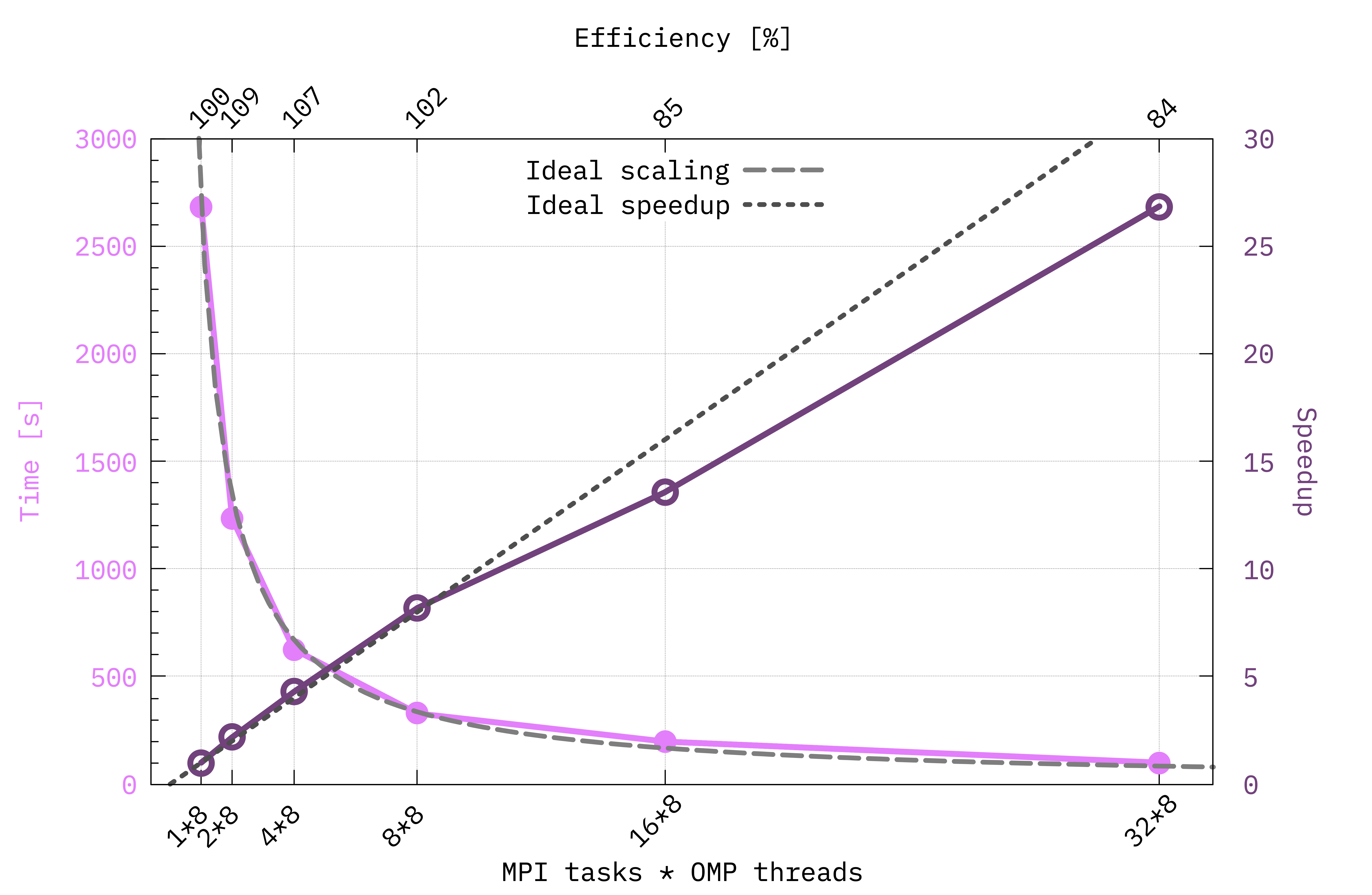
Example of scaling plot obtained running on GPUs with the parallelization scheme set by the script from before. Notice that here the number of OMP threads has been kept fixed to 8. In this case we can define the speedup corresponding to the calculation with \(N\) MPI tasks as \(\mathrm{time}(N=1) / \mathrm{time}(N)\) and the efficiency as the ratio between the real and the ideal speedup. The ideal trends are obtained if doubling the computational resources halves the time to solution.
Note
You are not supposed to get the same exact numbers in your plot, but you should get a similar trend.
Notice also that using the input parameters (number of bands for \(\chi\) and \(\Sigma\), energy cutoff, number of QP corrections etc.) as they are in the gw.in it takes around 45 minutes on 1 GPU for the calculation to finish.
Looking at the scaling plot what can we learn from it? Up to which number of MPI tasks our system scales efficiently? How can we decide at which point adding more nodes to the calculation becomes a waste of resources?
From this kind of plots we can learn a lot on how we should distribute the calculation so that it scales efficiently, thus avoiding to waste resources.
Comparing different parallelization schemes (optional)
As you can see from the choice of the variables DIP_CPU, X_and_IO_CPU and SE_CPU we made in the script from before, we have parallelized over a single parameter, i.e. c or qp, but Yambo allows for tuning the parallelisation scheme over several parameters broadly corresponding to “loops” (i.e., summations or discrete integrations) in the code.
For example, now we are calculating a lot of QP corrections (QPkrange is 1|19|23|30|, so 152 in total) so it makes sense to prioritize the parallelization over qp.
However in the cases where we only calculate two QP corrections (for example those corresponding to the fundamental gap of the system), we can put at most 2 in correspondence of qp.
In this case the parallelization over b (that is bands) is very useful.
You may open again the run_parallel.sh script and modify the section where the Yambo input variables are set.
For example, X_CPU sets how the MPI Tasks are distributed in the calculation of the response function.
The possibilities are shown in the X_ROLEs.
The same holds for SE_CPU and SE_ROLEs which control how MPI tasks are distributed in the calculation of the self-energy.
X_CPU= "1 1 1 $ncpu 1"      # [PARALLEL] CPUs for each role
X_ROLEs= "q g k c v"        # [PARALLEL] CPUs roles (q,g,k,c,v)
X_nCPU_LinAlg_INV= $ncpu    # [PARALLEL] CPUs for Linear Algebra
X_Threads=  0               # [OPENMP/X] Number of threads for response functions
DIP_Threads=  0             # [OPENMP/X] Number of threads for dipoles
SE_CPU= "1 $ncpu 1"         # [PARALLEL] CPUs for each role
SE_ROLEs= "q qp b"          # [PARALLEL] CPUs roles (q,qp,b)
SE_Threads=  0              # [OPENMP/GW] Number of threads for self-energy
You can try different parallelization schemes and check the performances of Yambo.
Don’t forget that the product of the numbers entering each variable (i.e. X_CPU and SE_CPU) times the number of threads should always match the total number of cores (unless you want to overload the cores taking advantage of multi-threads).
Caution
You should also change the -J and -C flags through label=MPI${ncpu}_OMP${nthreads} in the run_parallel.sh script to avoid confusion with previous calculations.
You may then check how speed, memory and load balance between the CPUs are affected, adapting the script parse_ytiming.py to parse the new data, read and distinguish between more file names, new parallelisation options, etc.
Tip
Memory scales better if you parallelize on bands (
c,v,b).Parallelization over k-points (
k) performs similarly to parallelization on bands, but requires more memory.Parallelization over q-points (
q) requires much less communication between the MPI tasks. It may be useful if you run on more than one node and the inter-node connection is slow.
Performance of Yambo on large systems
Benchmarks performed on large-scale simulations show that Yambo scales very well up to thousands of MPI tasks combined with OpenMP parallelism, retaining good efficiency even in highly parallelized calculations.
These benchmarks have been run on several supercomputers all around the world[1]. For example, take a look at the performance on the Fugaku supercomputer in Japan (see also this post), Leonardo in Italy, LUMI in Finland.
Full GW band structure (optional)
Now that we are familiar with the parallelization schemes of a GW calculation, let’s put into practice what we have learned with a more realistic scenario: the calculation of a full band structure with (kind of) converged parameters.
For this step we increased the vacuum separation (to 30 au) and the k-point mesh (to 18x18x1) in the DFT calculation, we included spin-orbit coupling and, concerning the GW part, we set more balanced parameters for the number of bands and energy cutoff. In addition, we want to compute QP corrections on the entire Brillouin zone, for two spin-orbit-split valence bands and two spin-orbit-split conduction bands.
Go to the 04_GW_bands folder:
$ cd MoS2_HPC_tutorial/04_GW_bands
and inspect the input file gw.in.
The most relevant parameters that determine how we should parallelize the calculation in this case are the following:
[...]
% BndsRnXp
   1 | 100 |      # [Xp] Polarization function bands
%
NGsBlkXp= 5   Ry  # [Xp] Response block size
[...]
% GbndRnge
   1 | 100 |      # [GW] G[W] bands range
%
[...]
%QPkrange         # [GW] QP generalized Kpoint/Band indices
1|37|25|28|
%
Note
If you want you can use the screening databases (and other available databases) corresponding to these parameters provided in the GW_bnds folder, namely
$ ls GW_bnds/ndb.pp*
GW_bnds/ndb.pp
GW_bnds/ndb.pp_fragment_1
[...]
GW_bnds/ndb.pp_fragment_37
You can do this running Yambo with -J GW_bnds.
Attention
If you decide to change some of the input variables, chances are that you need to compute new databases.
For example if you change the value of NGsBlkXp (either increasing or reducing it), the GW_bnds/ndb.pp* databases cannot be used anymore.
A safer option is to specify a new folder to print any new databases, e.g. -J GW_bnds_new,GW_bnds.
In this way Yambo will look for compatible databases in all the folders (starting from the first one) and print newly computed ones in the first one in case it does not find any.
In this calculation we have 100 bands (27 of which are occupied and the rest empty, as you may verify running a quick setup), 37 k-points, a 5 Ry energy cutoff for the dielectric matrix and 148 quasiparticle corrections.
With this information (and knowing the machine where you are going to run this calculation) set the parallelization variables in the input file gw.in
DIP_CPU= "1 1 1"              # [PARALLEL] CPUs for each role
DIP_ROLEs= "k c v"            # [PARALLEL] CPUs roles (k,c,v)
DIP_Threads=  0               # [OPENMP/X] Number of threads for dipoles
X_and_IO_CPU= "1 1 1 1 1"     # [PARALLEL] CPUs for each role
X_and_IO_ROLEs= "q g k c v"   # [PARALLEL] CPUs roles (q,g,k,c,v)
X_Threads=  0                 # [OPENMP/X] Number of threads for response functions
SE_CPU= "1 1 1"               # [PARALLEL] CPUs for each role
SE_ROLEs= "q qp b"            # [PARALLEL] CPUs roles (q,qp,b)
SE_Threads=  0                # [OPENMP/GW] Number of threads for self-energy
and adjust your submission script file accordingly before submitting the job.
When the calculation is done we find the quasiparticle corrections stored in human-readable form in the file o-*.qp inside the output directory (the * being replaced by the -J label you chose), and in netCDF format in the quasiparticle database ndb.QP inside the job directory.
In order to visualize the results in the form of a GW band structure, we will first interpolate the calculated points - recall that we have just 37 points, few of which lie on high-symmetry lines - with ypp, the yambo pre- and post-processing executable.
Tip
You can do this also with Yambopy.
To generate the ypp input file for band structure interpolation type
$ ypp -s b -F ypp_bands.in
(as with yambo, you can see all the available options with ypp -h).
Attention
You may need open an interactive session to run ypp.
Let us modify the resulting input file by selecting the boltztrap approach to interpolation, the last two valence and first two conduction bands, a path in the Brillouin zone along the the points \(\Gamma - M - K - \Gamma\) and 100 points for each high-symmetry line:
electrons                        # [R] Electronic properties
bnds                             # [R] Bands
PROJECT_mode= "none"             # Instruct ypp how to project the DOS. ATOM, LINE, PLANE.
INTERP_mode= "BOLTZ"             # Interpolation mode (NN=nearest point, BOLTZ=boltztrap aproach)
INTERP_Shell_Fac= 20.00000       # The bigger it is a higher number of shells is used
INTERP_NofNN= 1                  # Number of Nearest sites in the NN method
OutputAlat= 5.90008              # [a.u.] Lattice constant used for "alat" ouput format
cooIn= "rlu"                     # Points coordinates (in) cc/rlu/iku/alat
cooOut= "rlu"                    # Points coordinates (out) cc/rlu/iku/alat
% BANDS_bands
   25 | 28 |                     # Number of bands
%
CIRCUIT_E_DB_path= "none"        # SAVE obtained from the QE `bands` run (alternative to %BANDS_kpts)
BANDS_path= ""                   # High-Symmetry points labels (G,M,K,L...) also using composed positions (0.5xY+0.5xL).
BANDS_steps= 100                 # Number of divisions
#BANDS_built_in                  # Print the bands of the generating points of the circuit using the nearest internal point
%BANDS_kpts                      # K points of the bands circuit
 0.00000 |0.00000 |0.00000 |
 0.00000 |0.50000 |0.00000 |
 0.33333 |0.33333 |0.00000 |
 0.00000 |0.00000 |0.00000 |
%
Run the calculation with
$ ypp -F ypp_bands.in
Attention
Use mpirun -np 1 ypp or mpiexec -np 1 ypp if needed on your machine.
This run will produce the file o.bands_interpolated.
You can inspect it and see that it contains a plottable band structure, but beware: these are the DFT eigevalues!
We didn’t tell ypp where to look for the quasiparticle corrections, so it went into the SAVE folder and interpolated the DFT data.
Let’s rename the output:
$ mv o.bands_interpolated o.DFT_bands
$ mkdir DFT_bands
$ mv o.spin* o.magn* DFT_bands/
In order to interpolate the quasiparticle energies, add the following line in the ypp input
GfnQPdb= "E < ./<your -J label>/ndb.QP"
and run ypp again as before.
When it’s done, rename the outputs as follows
$ mv o.bands_interpolated o.GW_bands
$ mkdir GW_bands
$ mv o.spin* o.magn* GW_bands/
You can now compare the DFT and GW bands by plotting them, using the plt_bands.gnu gnuplot script below if you want. If you prefer python, you can use the python script plt_bands.py that you will find in the tutorial directory (the latter script needs numpy and matplotlib).
plt_bands.gnu
### Terminal
set terminal qt persist enhanced font "Helvetica,12"

### Files
file_DFT = "o.DFT_bands"
file_GW  = "o.GW_bands"

### Axes & tics
set xrange [0:237]
set xtics ("{/Symbol G}" 0, "M" 87, "K" 137, "{/Symbol G}" 237)
set ylabel "Energy (eV)"
set grid xtics ytics
set border lw 1.5

### Line styles
set style line 1 lc rgb "#000000" lw 2   # DFT
set style line 2 lc rgb "#d62728" lw 2   # GW

### Legend
set key top right spacing 1.2

### Plot
plot \
    file_DFT u 0:2 w l ls 1 t "DFT", \
    file_DFT u 0:3 w l ls 1 notitle, \
    file_DFT u 0:4 w l ls 1 notitle, \
    file_DFT u 0:5 w l ls 1 notitle, \
    file_GW  u 0:2 w l ls 2 t "GW",  \
    file_GW  u 0:3 w l ls 2 notitle, \
    file_GW  u 0:4 w l ls 2 notitle, \
    file_GW  u 0:5 w l ls 2 notitle
Save this in a file named PLOT_bands.gnu and then load it in gnuplot to
plot the bands:
$ gnuplot
gnuplot> load 'PLOT_bands.gnu'
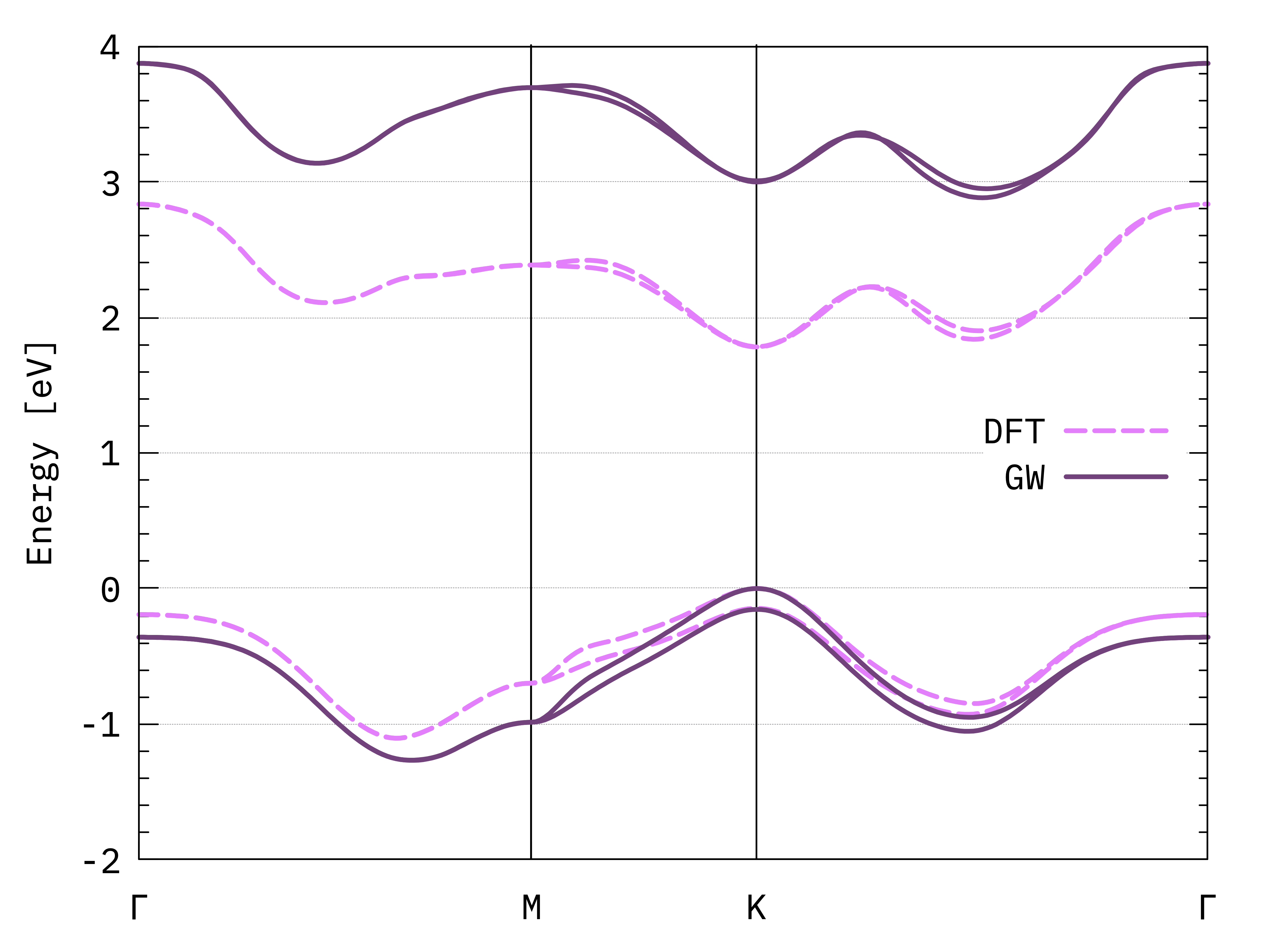
GW and DFT bands of monolayer MoS2.
You may compare this plot with a converged result, for example Fig. 10 of this article[2].
Note
The result obtained here is not too bad, but there are some differences both at the DFT and GW levels. The magnitude of the band gap is too large, and the relative energy of the two conduction band minima is not correct. One obvious issue is the lack of convergence of our tutorial calculation. As we know, we should include more vacuum space and many, many more k-points. Additionally, this is a transition metal dichalcogenide: for this class of systems, the details of the band structure can strongly depend on small variations in the lattice parameters and on the type of pseudopotential used.
A great deal of care must be taken when performing these calculations!