Optics at the independent particle level
In this tutorial you will learn the first steps for calculating optical properties with Yambo. In particular we will perform optics calculations at the independent particle (IPA) level for bulk hexagonal boron nitride (hBN).
Requirements
hBNfolder: download and extracthBN.tar.gzfrom the Tutorial files pagethe
SAVEfolder (present inhBN/YAMBO)yamboexecutablegnuplotfor plotting spectra
It is assumed that you are familiar with the concepts related to the SAVE folder and handling files with Yambo.
The dielectric function in the long-wavelength limit at the independent particle level (RPA without local fields) is essentially given by the following:
In practice, Yambo does not use this expression directly but solves the Dyson equation for the susceptibility \(\chi\) (see tutorial on local fields).
We will use bulk hBN as an example, so download and unpack the files
and then go to the YAMBO directory:
$ cd hBN/YAMBO
Remember that the first thing to do is to initialize the SAVE folder
(or check if it has been already initialized):
$ ls SAVE/ndb.*
No such file or directory
$ yambo
[...]
$ ls
SAVE  l_setup  r_setup
$ ls SAVE
SAVE/ndb.gops  SAVE/ndb.kindx [...]
Input file and parameters
We want to perform a IPA optical spectrum calculation: the option to
generate the input file is -optics c (or -o c).
Let’s also add the option to choose the input file name:
$ yambo -F yambo.in_IP -o c
Tip
Remember the yambo -h command to print all the available options.
Important
In the input file the independent particle approximation for the optics is indicated by
Chimod= "IP" # [X] IP/Hartree/ALDA/LRC/PF/BSfxc
Optics runlevel
For optical properties we are interested just in the long-wavelength limit \(\mathbf{q} \to 0\). This always corresponds to the first \(\mathbf{q}\)-point in the set of possible \(\mathbf{q} =\mathbf{k} - \mathbf{k}'\) points.
Set the following input variables in yambo.in_IP to:
 % QpntsRXd
  1 | 1 |                    # [Xd] Transferred momenta
 %
 ETStpsXd= 1001              # [Xd] Total Energy steps
Setting the range of the variable QpntsRXd to 1 | 1 selects
only the first \(\mathbf{q}\).
ETStpsXd instead selects the number of calculated frequencies:
a large value ensures a smooth spectrum.
We can now run the calculation, specifying a job label using the
-J option:
$ yambo -F yambo.in_IP -J Full
View l-Full_optics_dipoles_chi
 <---> [01] MPI/OPENMP structure, Files & I/O Directories
 <---> MPI assigned to GPU : 0
 <---> [02] CORE Variables Setup
 <---> [02.01] Unit cells
 <---> [02.02] Symmetries
 <---> [02.03] Reciprocal space
 <---> [02.04] K-grid lattice
 <---> Grid dimensions      :   6   6   2
 <---> [02.05] Energies & Occupations
 <---> [03] Transferred momenta grid and indexing
 <---> [04] Dipoles
 <---> [04.01] Setup: observables and procedures
 <---> [DIP] Database not correct or missing. To be computed
 <---> [x,Vnl] computed using 4 projectors
 <02s> R V P [g-space] |########################################| [100%] --(E) --(X)
 <02s> [WARNING] [r,Vnl^pseudo] included in position and velocity dipoles.
 <02s> [WARNING] In case H contains other non local terms, these are neglected
 <02s> [05] Optics
 <02s> [LA] SERIAL linear algebra
 <02s> [X-CG] R(p) Tot o/o(of R):    5499   52992     100
 <02s> Xo@q[1] |########################################| [100%] --(E) --(X)
 <02s> [06] Timing Overview
 <02s> [07] Memory Overview
 <02s> [08] Game Over & Game summary
Note
Yambo runs the calculation when there are no lowercase options after yambo.
When the calculation has finished you should see these files:
$ ls
 Full  SAVE  yambo.in_IP  r_setup  l_setup  l-Full_optics_dipoles_chi
 o-Full.eel_q1_ip  o-Full.eps_q1_ip  r-Full_optics_dipoles_chi
Let’s take a moment to understand what Yambo has done inside the Optics runlevel:
Compute the \([\mathbf{r}, V^\mathrm{NL}]\) term
Read the wavefunctions from disc
[WF]Compute the dipoles, i.e. matrix elements of \(\mathbf{p}\)
Write the dipoles to disk as
Full/ndb.dip*databases. You can check this from the report file:
$ grep -A16 "WR" r-Full_optics_*
grep output
[WR./Full//ndb.dipoles]---------------------------------------------------------
 Brillouin Zone Q/K grids (IBZ/BZ)                :   14   72   14   72
 RL vectors                                       :  1491 [WF]
 Fragmentation                                    : yes
 Electronic Temperature                           :  0.000000 [K]
 Bosonic    Temperature                           :  0.000000 [K]
 DIP band range                                   :    1  100
 DIP band range limits                            :   8   9
 DIP e/h energy range                             : -1.000000 -1.000000 [eV]
 RL vectors in the sum                            :  1491
 [r,Vnl] included                                 : yes
 Bands ordered                                    : yes
 Direct v evaluation                              : no
 Approach used                                    : G-space v
 Dipoles computed                                 : R V P [G-space]
 Wavefunctions                                    : Slater exchange(X)+Perdew & Zunger(C)
- S/N 003471 ---------------------------------------------- v.05.03.00 r.23927 -
$ grep -A16 "WR" r-Full_optics_*
grep output
[WR./Full//ndb.dip_iR_and_P]
Brillouin Zone Q/K grids (IBZ/BZ):  14   72   14   72
RL vectors                   (WF): 1491
Electronic Temperature        [K]: 0.0000000
Bosonic    Temperature        [K]: 0.0000000
X band range           :   1  100
RL vectors in the sum  : 1491
[r,Vnl] included       :yes
...
Finally, Yambo computes the non-interacting susceptibility \(\chi\) for this \(\mathbf{q}\), and writes the dielectric function inside the
o-Full.eps_q1_ipfile for plotting
Important
If yambo is computing new databases you will see WR. at the corresponding runlevel
in the report file. If yambo finds a compatible database, this will be read and you
will see RD. in place of WR..
This is useful to check wheter yambo is actually computing the database, especially
after you have changed some input variables.
Note on the energy cutoff
The previous calculation used all the G-vectors in expanding the wavefunctions, up to 1491 (~1016 components). This corresponds roughly to the cut off energy of 40 Ry we used in the DFT calculation.
Generally, however, we can use a smaller value. We use the verbosity to switch on this variable:
$ yambo -F yambo.in_IP -V RL -o c
Change the value of FFTGvecs and also its unit
from RL (number of G-vectors) to Ry (energy in Rydberg):
FFTGvecs= 6 Ry # [FFT] Plane-waves
Save the input file and launch the code again
with a new -J flag to avoid reading the
database from before:
$ yambo -F yambo.in_IP -J 6Ry
The result will be printed in the file o-6Ry.eps_q1_ip.
Caution
In general the best practice is to keep the value of FFTGvecs at its
default (maximum) value.
Plotting the output
To plot the result in o-Full.eps_q1_ip file type:
$ gnuplot
gnuplot> plot "o-Full.eps_q1_ip" w l
The figure below also shows the results with lower energy cutoff.
If you also did this calculation you can add the plot on top of
the previous one with replot "o-6Ry.eps_q1_ip" w p.

Comparison between the IPA dielectric functions in the long-wavelenght limit, i.e. \(\Im(\varepsilon_{\alpha,\alpha}(\omega))\) (Eq.(1)), computed with the total number available G-vectors (Full) and a cutoff value of 6 Ry.
Note
In this case the direction of the electric field (i.e. \(\alpha,\alpha\)) is the one of the lattice vector \(\boldsymbol{\mathrm{a}}\) of the unit cell – which is also parallel to the \(x\) axis – because in the input file we have
% LongDrXd
 1.000000 | 0.000000 | 0.000000 |        # [Xd] [cc] Electric Field
%
Important
We can see that there is very little difference between the two spectra.
This highlights an important point in calculating excited state properties:
generally, fewer G-vectors are needed than what are needed in DFT calculations.
However we suggest to never change the value of FFTGvecs (unless you have
very limited memory, in which case carefully check how changing this value
affects the results).
Regarding the spectrum itself, the first peak occurs at about 4.4 eV. This is consistent with the minimum direct gap reported by Yambo: 4.28 eV. The comparison with experiment (not shown) is very poor however. This is because in most materials more advanced techniques than IPA/RPA are needed.
q-direction
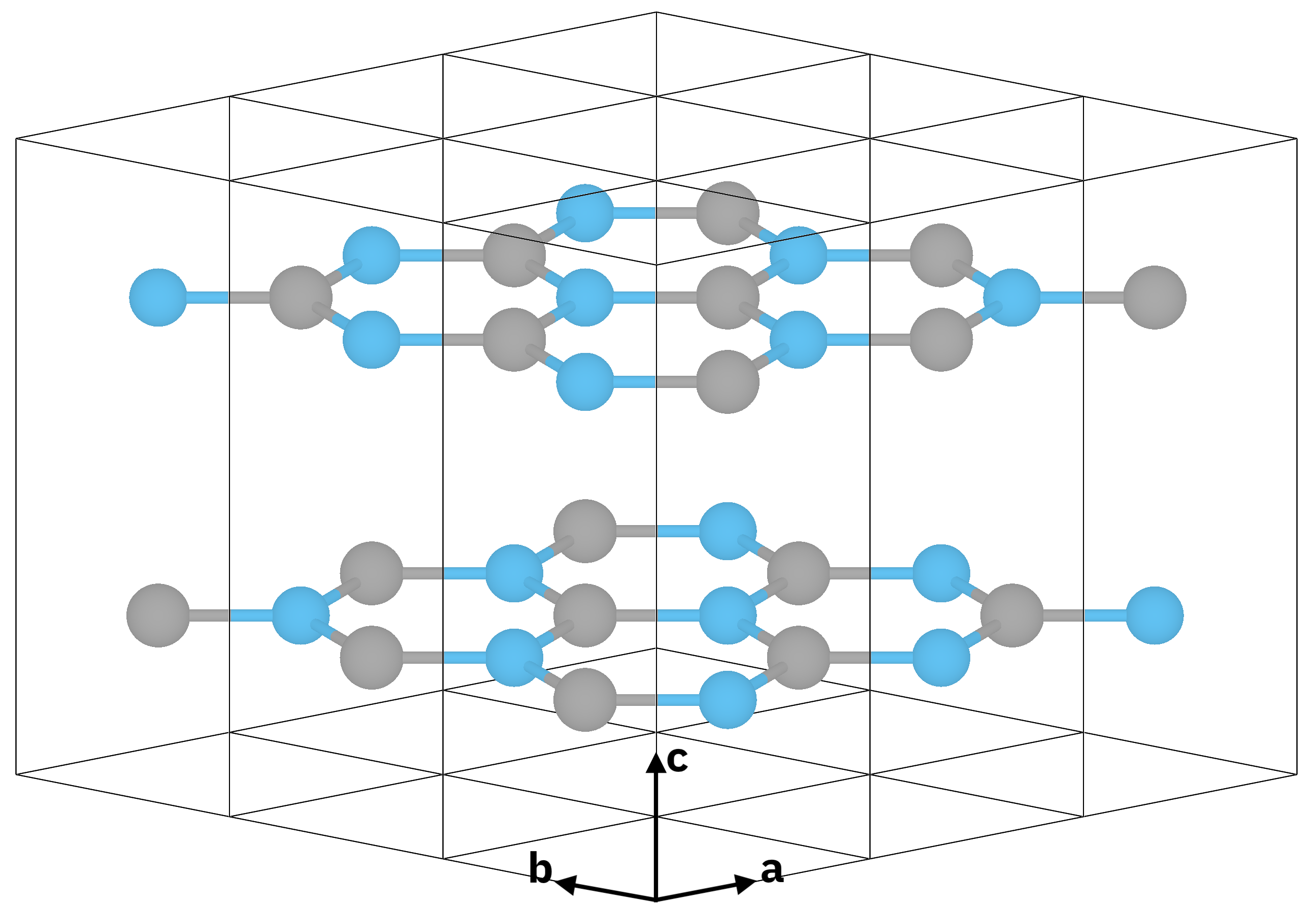
Atomic structure of bulk hBN (\(z \parallel c\) is the stacking direction).
Now let’s do the calculation for the \(\epsilon_{z,z}(\omega)\)
component of the dielectric tensor. To do so we modify LongDrXd
in the input file
$ yambo -F yambo.in_IP -o c
...
% LongDrXd
0.000000| 0.000000 | 1.000000 |        # [Xd] [cc] Electric Field
%
...
and run the calculation again
$ yambo -F yambo.in_IP -J Full
This time yambo reads from the Full folder, so it does not need to compute
the dipole matrix elements again and the calculation is faster.
Let’s plot the result:
$ gnuplot
gnuplot> plot "o-Full.eps_q1_ip" t "q || x-axis" w l,"o-Full.eps_q1_ip_01" t "q || z-axis" w l
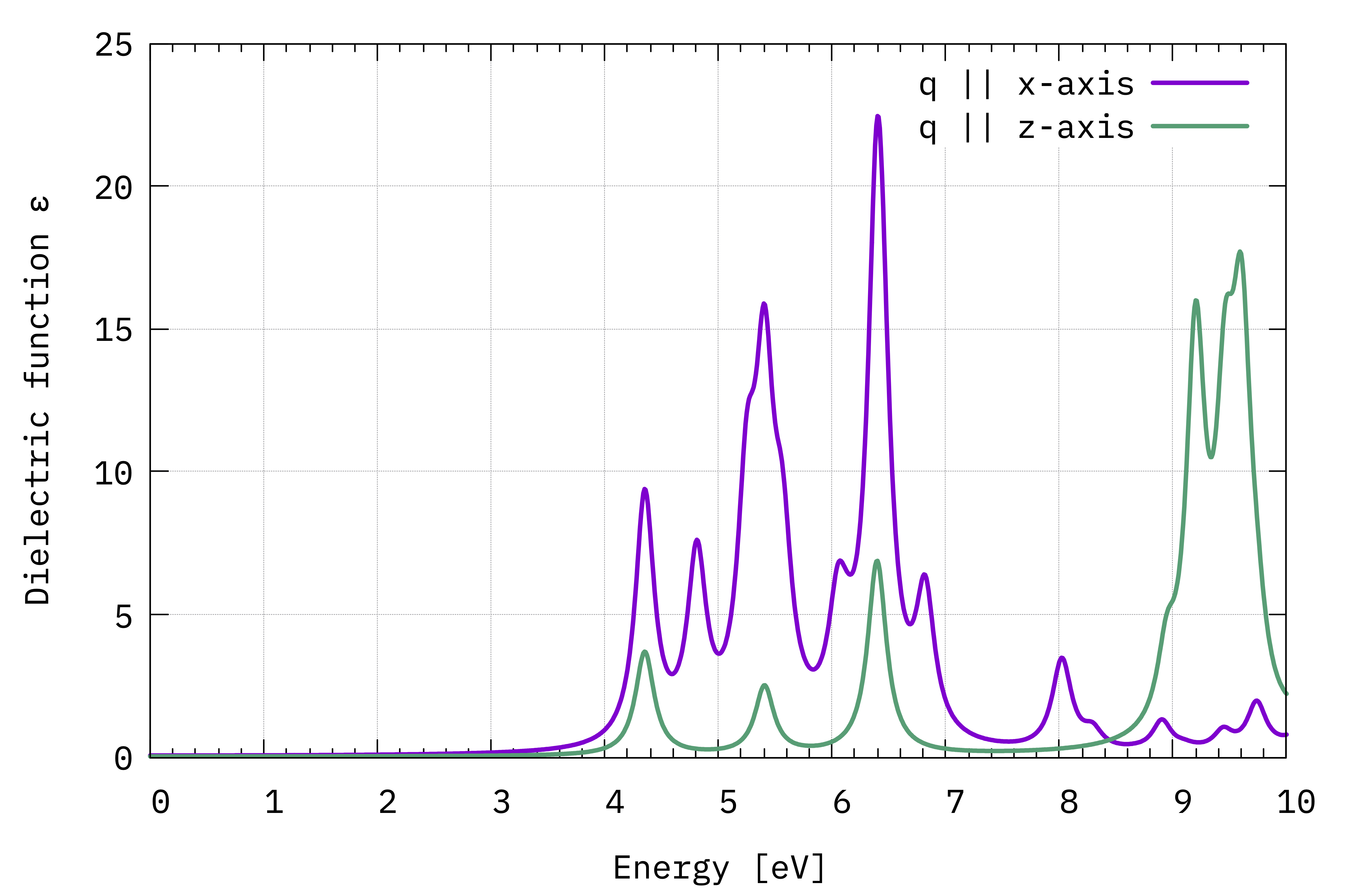
Comparison between \(\Im(\varepsilon_{x,x}(\omega))\) and \(\Im(\varepsilon_{z,z}(\omega))\) (Eq.(1)).
The absorption is suppressed in the stacking direction. As the interplanar spacing is increased, we would eventually arrive at the absorption of the BN sheet (see local fields tutorial).
Non-local commutator
Last, we show the effect of switching off the non-local commutator term (the term with \(V^\mathrm{NL}\) in Eq. (1)) due to the pseudopotential.
As there is no option to do this inside Yambo, you need to hide the database file, for example renaming it like this:
$ mv SAVE/ns.kb_pp_pwscf SAVE/ns.kb_pp_pwscf_OFF
Then open the input file and modify it back to do the calculation along the \(q \parallel (1 0 0)\) direction
 % LongDrXd
 1.000000  | 0.000000 |  0.000000  |
 %
and launch yambo with a different -J label:
$ yambo -F yambo.in_IP -J Full_NoVnl
Important
Note the warning in the log:
<---> [WARNING] [r,Vnl^pseudo] not included in position and velocity dipoles
which also appears in the report file r-Full_NoVnl_optics_dipoles_chi as
[WR./Full_NoVnl//ndb.dipoles]----------------------------------------------------
 ...
 [r,Vnl] included                                 : no
 ...
Plotting the result we see that the difference is small:
$ gnuplot
gnuplot> plot "o-Full.eps_q1_ip" w l t "w/ Vnl", "o-Full_NoVnl.eps_q1_ip" w p t "no Vnl"
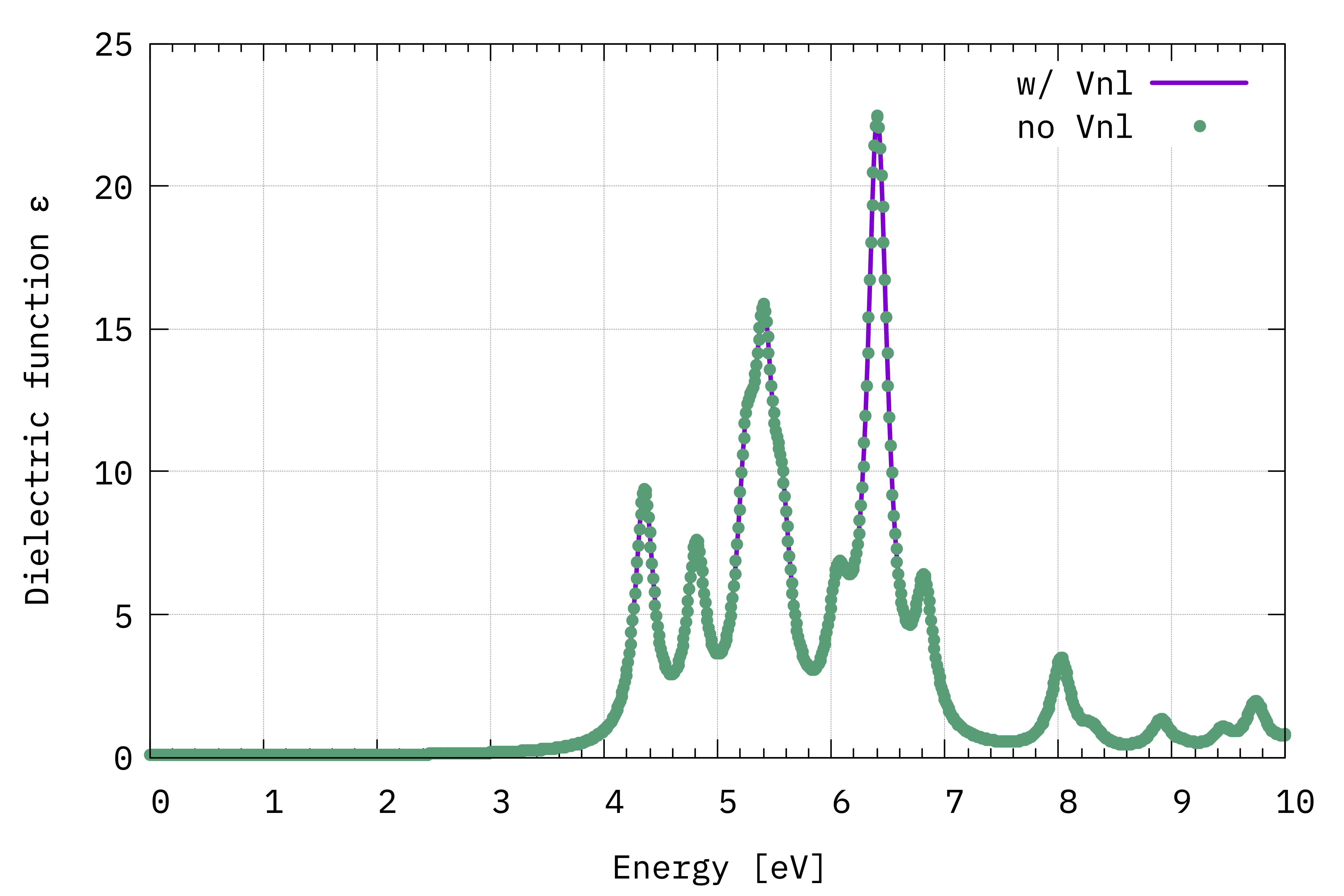
Comparison between \(\Im(\varepsilon_{x,x}(\omega))\) computed with and without the \(V^{\mathrm{NL}}\) term (Eq.(1)).
Tip
When you have a large system, either with more projectors in the pseudopotential or more k-points, the inclusion of \(V^\mathrm{NL}\) can make a huge difference in the computational load. So it is always worth checking to see if these terms are important for your system.