Database generation¶

In this tutorial you will learn how to generate the SAVE folder starting from a Quantum ESPRESSO calculation. Notice that beyond Quantum ESPRESSO other DFT codes can be used to generate wave-functions for Yambo, namely Abinit and PWmat.

Requirements

hBN folder: download and extract hBN.tar.gz from the Tutorial files page
pw.x executable (version 5.0 or newer)
p2y and yambo executables

After you have downloaded the required files, move to the hBN folder:

$ cd hBN/
$ ls
COPYING  PWSCF  README.tutorials  YAMBO

The following structure is common to various tutorials: a PWSCF folder containing all the files related to the starting DFT calculation (including pseudopotentials and reference output files) and a YAMBO folder for the Yambo calculations.

Before we begin with the tutorial, here are some useful information specific to the example of bulk hBN:

HCP lattice, ABAB stacking
Four atoms per cell, B and N (16 electrons)
Lattice constants: a = 4.716 [a.u.], c/a = 2.582
Plane wave cutoff: 40 Ry (~1500 RL vectors in wavefunctions)
SCF: shifted 6x6x2 grid (12 k-points), 8 bands
Non-SCF run: gamma-centered 6x6x2 grid (14 k-points), 100 bands

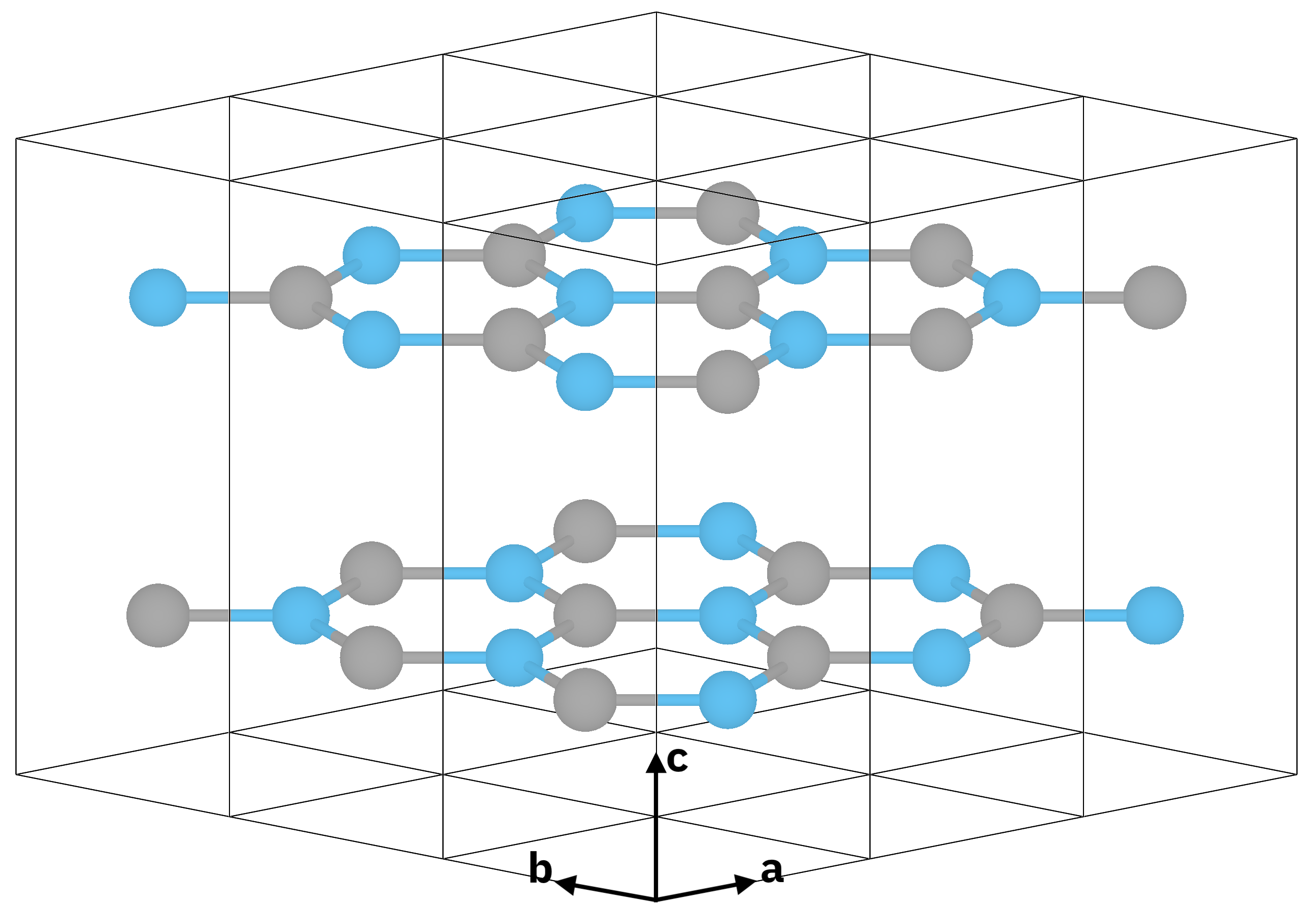
../../_images/hBN-bulk-3x3.png — Atomic structure of bulk hexagonal boron nitride (hBN).¶

Note

2D hexagonal lattice
Two atoms per cell, B and N (8 electrons)
Lattice constants: a = 4.716 [a.u.], c/a = 7
Plane wave cutoff: 40 Ry (~5000 RL vectors in wavefunctions)
SCF: shifted 6x6x1 grid (12 k-points), 4 bands
Non-SCF run: gamma-centered 6x6x1 grid (7 k-points), 60 bands

../../_images/hBN-2D-3x3.png — Atomic structure of 2D hBN.¶

In the case of 2D hBN there is only one layer and the lattice constant along z is set to c/a = 7 (to add sufficient vacuum). Notice that because of the added vacuum the same plane wave energy cutoff of 40 Ry will correspond to ~5000 RL vectors. This is relevant because in Yambo you can specify energy cutoff values either in Ry or RL.

DFT calculations¶

Go to the PWSCF folder:

$ cd hBN/PWSCF
$ ls
Inputs  Pseudos  References  hBN_nscf.in  hBN_nscf_bands.in  hBN_plot_bands.in  hBN_scf.in  hBN_scf_bands.in

Warning

The output of ls may be different in case the tutorial files are updated.

Now run the SCF calculation to generate the ground-state charge density, occupations, and so on:

$ pw.x < hBN_scf.in > hBN_scf.out

Looking at the output file we can see that the valence band maximum lies at 5.06 eV.

Next run a non-SCF calculation to generate a set of Kohn-Sham eigenvalues and eigenvectors for both occupied and unoccupied states:

$ pw.x < hBN_nscf.in > hBN_nscf.out

In this calculation we computed a total of 100 bands (nbnd = 100 in the input file) and used a 6x6x2 grid (corresponding to 14 k-points).

Notice the presence of the following flags in the input file:

wf_collect       = .true.
force_symmorphic = .true.
diago_thr_init   = 5.0e-6,
diago_full_acc   = .true.

These are needed for generating the Yambo databases accurately. If you are not familiar with pw.x input variables you can find a full and detailed explanation on the pw.x input description page.

Note

The wf_collect input variable is actually deprecated, but its inclusion in the input does not give any problems.

These calculations produce the hBN.save folder, which is needed by p2y:

$ ls hBN.save
B.pz-vbc.UPF N.pz-vbc.UPF charge-density.dat data-file-schema.xml wfc1.dat wfc2.dat wfc3.dat wfc4.dat ... wfc14.dat

Conversion to Yambo format¶

The hBN.save output folder is converted to the Yambo format using the p2y executable (pwscf to yambo). Launch p2y from inside the hBN.save folder:

$ cd hBN.save
$ p2y

Tip

If you run p2y in background or via some job submission script the log information will be printed in a l_p2y file.

You can see that p2y has generated the SAVE folder:

$ ls SAVE
ns.db1 ns.wf ns.kb_pp_pwscf ns.kb_pp_pwscf_fragment_1 ns.kb_pp_pwscf_fragment_2 ... ns.kb_pp_pwscf_fragment_14 ns.wf_fragments_1_1 ... ns.wf_fragments_14_1

These files, with an n prefix, indicate that they are in netCDF format, and thus not human readable. However they are perfectly transferable across different architectures. You can check that the databases contain the information you expect by launching yambo using the -D option:

$ yambo -D

Note

The layout of the text may be different in other versions of Yambo.

When you do your calculations we suggest to move the SAVE folder into a new clean folder. Concerning the tutorials, typically there is already a SAVE folder in the YAMBO directory.