BSE on MoS2: solvers
In this tutorial we will focus on the solution of the BSE equation. We will use 2D MoS2 as an example system.
Requirements
SAVEfolder of 2D MoS2: download and extractMoS2_HPC_BSE_tutorial.tar.gzfrom the Tutorial files pageGW_bnds(optional): folder containing quasiparticle databases from GW calculation and precomputed RPA screeningyamboexecutablegnuplot(optional) for plotting some of the resultsxcrysdenorVESTA(optional) to visualize exciton wavefunctions
It is assumed that you are familiar with the concepts related to the SAVE folder and handling files with Yambo.
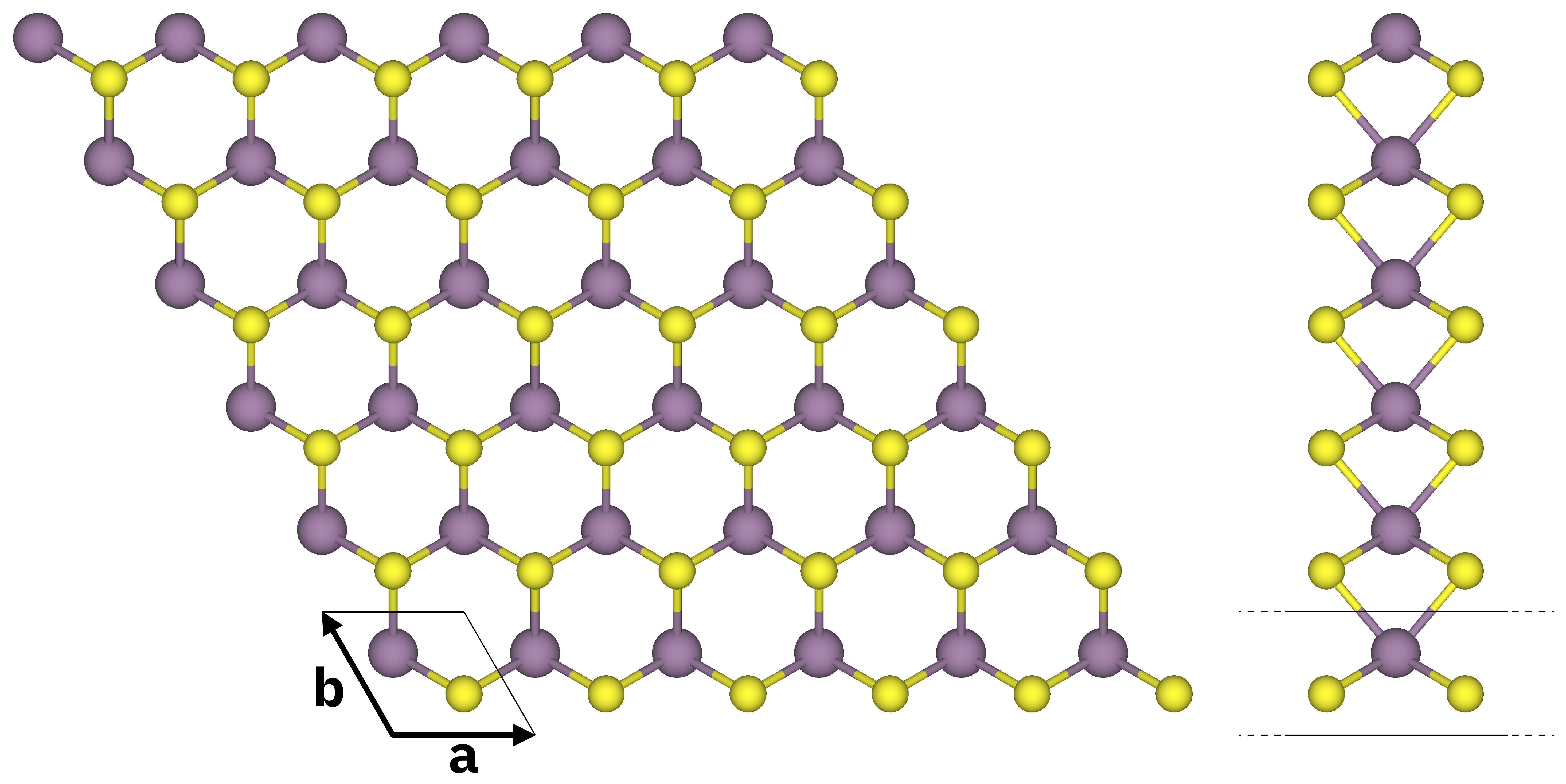
Atomic structure of monolayer MoS2 (top and side views). S atoms in yellow, Mo atoms in purple. The solid black lines mark the unit cell.
Quick overview
Yambo is run on top of DFT results, in this case from the code Quantum ESPRESSO (QE).
The “step 0” of every calculation is converting this directory to yambo-readable format via the p2y interface, but here it is skipped.
The SAVE folder is already present in 01_BSE_Hamiltonian (where you will start the tutorial).
The SAVE directory contains:
crystal lattice information in real and reciprocal space
pseudopotential information
DFT-computed electron energies
DFT-computed electron wavefunctions
These data are the DFT starting point to the many-body perturbation theory simulations.
In addition, while a BSE calculation can be run on top of DFT results, from a theoretical point of view this should be done on top of a GW calculation to maintain consistency of methods used.
For this tutorial, you can use the databases for quasiparticle energies and RPA screening already calculated during the GW on MoS2 tutorial.
These databases are provided in 01_BSE_Hamiltonian/GW_bnds:
ndb.QPdatabase with quasiparticle energiesndb.pp*databases with static RPA microscopic dielectric functionndb.RIM,ndb.cutoffdatabases concerning the Coulomb potential integration in 2D (since we are dealing with a 2D system).
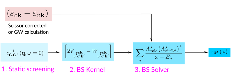
The target quantity in a Bethe-Salpeter calculation is the macroscopic dielectric matrix \(\epsilon_{M}\). The following quantities/steps are needed to obtain \(\epsilon_{M}\):
Build the excitonic Hamiltonian
To solve the Bethe–Salpeter equation (BSE), it is customary to rewrite it in the basis of transitions between valence and conduction states. In this representation, the problem takes the form of an eigenvalue equation for an effective two-particle Hamiltonian. For a non–spin-polarized system and in the optical limit \(q=0\), the matrix elements of the two-particle Hamiltonian are given by:
where \(vck\) indicates the pair of quasiparticle states \(vk\) and \(ck\) (that is, an electron-hole transition from the valence band to the conduction band with momentum \(\mathbf{k}\)). Quasiparticle energies are either calculated from a previous GW calculation or approximated by the Kohn-Sham energies (calculated at DFT level) corrected via a scissor operator.
The first term on the RHS is given by the quasiparticle energy differences (diagonal only). The second term is the kernel, which is the sum of the electron-hole exchange part \(V\) – which stems from the Hartree potential and has a repulsive effect – and the electron-hole attraction part \(W\) – which stems from the screened exchange potential: this term is attractive and it is responsible for the binding of electron-hole pairs. The electron-hole interaction kernel both shifts (diagonal contributions) and couples (off-diagonal contributions) the quasiparticle energy differences.
The kernel contributions are built up by calculating the following expressions:
Here \(\epsilon^{-1}_{{\bf G}{\bf G}'}\) is the inverse of the dielectric screening matrix which was evaluated at the RPA level.
Yambo input file
We now generate the input file needed to build the BSE kernel.
This is done using the yambo executable with the following command-line instruction:
$ cd MoS2_HPC_BSE_tutorial/01_BSE_Hamiltonian/
$ yambo -o b -X p -k sex -r -F bse.in -V par -J GW_bnds
(remember yambo -h for the full list of options).
With these options we generate an input file for a Bethe-Salpeter optics calculation (-o b), using the RPA screening from a plasmon-pole calculation (-X p) and using the Hartree-Screened exchange kernel (-k sex).
We also add a truncation of the Coulomb potential which is useful for 2D systems (-r).
In addition, we want to set up explicitly the parameters for parallel runs, so we use -V par.
In order to include quasiparticle energies we could specify -V qp, but this switches on many variables, most of which we don’t need to change.
Thus we will add manually the only one that we need, i.e. KfnQPdb.
You can now inspect the input file bse.in and try to familiarize with some of the parameters.
Note
Since we have specified -J GW_bnds, some input file variables are automatically set compatibly with the databases found in GW_bnds.
Let us quickly review and set the relevant parameters for our case.
Runlevels
optics         # [R] Linear Response optical properties
ppa            # [R][Xp] Plasmon Pole Approximation for the Screened Interaction
rim_cut        # [R] Coulomb potential
bse            # [R][BSE] Bethe Salpeter Equation.
dipoles        # [R] Oscillator strenghts (or dipoles)
em1d           # [R][X] Dynamically Screened Interaction
These flags tell Yambo which parts of the code should be executed. Each runlevel enables its own set of input variables. Here we have:
optics: this is a calculation of optical properties…bse: …with the bse kernel;dipoles: dipoles are needed to build the kernel;em1dandppa: even if the BSE kernel just needs a static screening, we can use the previously calculated screening at plasmon-pole level as it contains the static limit at \(\omega=0\).
Bethe-Salpeter Hamiltonian
The relevant input variables to be set are:
BSENGexx=  20 Ry    # [BSK] Exchange components
BSENGBlk=  5  Ry    # [BSK] Screened interaction block size [if -1 uses all the G-vectors of W(q,G,Gp)]
% BSEBands
 23 | 30 |          # [BSK] Bands range
%
BSENGexx: cutoff on the summations over reciprocal lattice vectors for the bare exchange interaction \(V\);BSENGBlk: cutoff on the summations over reciprocal lattice vectors for the screened interaction \(W\);BSEBands: range of quasiparticle states – identified by their band indices – that defines the basis of electron–hole pairs used to describe excitonic states in the chosen energy window.
In our case, since the system has 26 occupied bands, we select bands 23–30, corresponding to four valence and four conduction bands. This choice leads to a total of 4×4=16 valence–conduction band pairs.
For each of these band pairs, all k-points available from the underlying DFT calculation are included.
With a 18×18×1 Monkhorst–Pack grid, this corresponds to 324 total k-points in the Brillouin zone.
As a result, the excitonic Hamiltonian is represented in a basis of 16×1296=5184 valence–conduction–k (vck) pairs: this is the dimension of the matrix.
Attention
The values chosen for these three parameters should be determined through systematic convergence studies.
RPA screening and Coulomb interaction
These parameters should be automatically filled in because they are read from the databases inside GW_bnds:
RandQpts= 1000000                # [RIM] Number of random q-points in the BZ
RandGvec= 109              RL    # [RIM] Coulomb interaction RS components
CUTGeo= "slab z"                 # [CUT] Coulomb Cutoff geometry: box/cylinder/sphere/ws/slab X/Y/Z/XY..
[...]
Chimod= "HARTREE"                # [X] IP/Hartree/ALDA/LRC/PF/BSfxc
[...]
% BndsRnXp
   1 | 100 |                           # [Xp] Polarization function bands
%
NGsBlkXp= 177              RL          # [Xp] Response block size
% LongDrXp
 0.707107E-5 | 0.707107E-5 |  0.00000  # [Xp] [cc] Electric Field
%
PPAPntXp= 27.21138         eV          # [Xp] PPA imaginary energy
Quasiparticle energies
Add the following line in the input to specify where to get quasiparticle energies:
KfnQPdb= "E < GW_bnds/ndb.QP"
KfnQPdb: this variable tells Yambo to look for the databasendb.QPthat contains quasiparticle energies from a previous GW calculations. These will be included in the BSE run.
Attention
Always specify this input variable, even if your ndb.QP database is in the SAVE folder, otherwise Yambo will use DFT eigenvalues.
Parallelization parameters
Finally, we need to choose the variables related to the parallelism:
BS_CPU= "1 1 1"        # [PARALLEL] CPUs for each role
BS_ROLEs= "k eh t"     # [PARALLEL] CPUs roles (k,eh,t)
For this run it is suggested to parallelize over k-points and in transition space. Different schemes may work best for different system sizes.
There is no need to set the parallelization parameters for dipoles and RPA response function: since they have already been calculated, the code will simply load the databases.
We are ready to run the kernel calculation: inspect the script run_bse.sh and submit it when you are satisfied.
Important
Make sure that the resources you required in the submission script match the ones you set in the input file.
Note
With the parameters reported above, the calculation takes around 15 minutes on 1 GPU.
In the report r-*_optics_dipoles_bse you will find the information related to this runlevel under the section:
[05] Bethe Salpeter Equation @q1
================================
Take some time to inspect the log and the report. For example try to find where the input parameters are reported, the dimension of the two-particles Hamiltonian and if these match your expectations.
This run does not produce any human readable output.
The kernel is stored in a database in the output BSE directory:
$ ls BSE/ndb*
BSE/ndb.BS_head_Q1  BSE/ndb.BS_PAR_Q1
Solve the excitonic Eigenvalue Problem
Now we move in the next directory for the diagonalization of the BSE Hamiltonian:
$ cd ../02_BSE_diagonalization
The eigenvalue equation reads:
From the solution of the eigenvalue problem it is possible to build the macroscopic dielectric function, from which the absorption and electron energy loss (EELS) spectra can be computed.
Those are obtained from the eigenvalues \(E^\lambda\) (excitonic energies) and eigenvectors \(A^\lambda_{cvk}\) (exciton composition in terms of electron-hole pairs) of the two-particle Hamiltonian:
Here you will have to adapt the submission script run_bse_diago.sh to your specific case.
First, we link the previously calculated databases to the current directory, so that they are available:
$ ln -s ../01_BSE_Hamiltonian/SAVE .
$ ln -s ../01_BSE_Hamiltonian/GW_bnds .
$ ln -s ../01_BSE_Hamiltonian/BSE .
Next, copy the input file from before in a new file bse_solver.in:
$ cp ../01_BSE_Hamiltonian/bse.in bse_solver.in
Before continuing, we must add the bss runlevel in bse_solver.in
[...]
bse               # [R][BSE] Bethe Salpeter Equation.
dipoles           # [R] Oscillator strenghts (or dipoles)
em1d              # [R][X] Dynamically Screened Interaction
bss               # [R] BSE solver
[...]
as well as the following lines to specify the parameters for the absorption spectrum (energy range, peak broadening, energy points and polarization direction of the absorbed electric field):
% BEnRange
  1.00000 | 5.00000 |        eV    # [BSS] Energy range
%
% BDmRange
 0.0500000 | 0.0500000 |     eV    # [BSS] Damping range
%
BEnSteps= 500                      # [BSS] Energy steps
% BLongDir
 1.000000 | 1.000000 | 0.000000 |  # [BSS] [cc] Electric Field versor
%
(you may add them at the end of the file).
Now we will explore three different ways to solve the excitonic matrix, namely:
the iterative
haydocksolvera direct diagonalization
the iterative
slepcsolver
To do this we will update the BSE input in three different ways.
1 Haydock iterative solver
The Haydock solver is an iterative method based on Lanczos chains. It is the fastest algorithm to obtain optical spectra, but it does not give access to the eigenvalues and eigenvectors of the excitonic Hamiltonian.
Copy the bse_solver.in file into bse_haydock.in
$ cp bse_solver.in bse_haydock.in
and then add the variables relative to the solver.
[...]
BSSmod= "h"            # [BSS] (h)aydock/(d)iagonalization/(s)lepc/(i)nversion/(t)ddft`
BSHayTrs=0.010000      # [BSS] Relative [o/o] Haydock threshold. Strict(>0)/Average(<0)
[...]
2 Full diagonalization of the excitonic Hamiltonian
This is the slowest algorithm, and it provides access to all eigenvalues and eigenvectors.
Let us create a different input by copying bse_haydock.in to bse_diago.in:
$ cp bse_solver.in bse_diago.in
In the new file, simply set the variable
BSSmod= "d" # [BSS] (h)aydock/(d)iagonalization/(s)lepc/(i)nversion/(t)ddft`
3 SLEPC iterative solver
In practical calculations, usually, only a fraction of the eigenvalues is significant to determine the optical properties of the material. The SLEPC library allows to do this via iterative schemes based on Krylov-Schur or Jacobi-Davidson methods (the default setting is Krylov-Schur). Create a third input file
$ cp bse_solver.in bse_slepc.in
and set the following input variables:
BSSmod="s"            # [BSS] (h)aydock/(d)iagonalization/(s)lepc/(i)nversion/(t)ddft`
BSSNEig=10            # [SLEPC/DIAGO] Number of eigenvalues to compute
The BSSNEig variable indicates the requested number of eigenvalues (and eigenvectors).
Important
Finally, we need to switch on the variable that writes the BSE eigenvectors to disk, which therefore only works when computing eigenvectors.
Add the following line in bse_diago.in and bse_slepc.in:
WRbsWF # [BSS] Write to disk excitonic the WFs
The eigenvectors are needed for post-processing purposes (such as plotting the exciton wavefunction in real space) and will be used in the following.
Note
WRbsWF is already present in the input if you generate it with the -Ksolver flag, but by default it is commented.
Keep in mind that WRbsWF writes the BSE eigenvectors to disk also in the case of the full diagonalization BSSmod= "d"
The script run_bse_diago.sh will run in sequence the three calculations related to the inputs we have prepared.
After adapting it to the specifics of your system, run the calculations.
If we check inside the absorption_* directories, we will find the relative output o-* output files.
When all the calculations are done, we have
$ ls -l absorption_*/o-*
absorption_diago/o-absorption_diago.alpha_q1_diago_bse
absorption_diago/o-absorption_diago.GW_bnds.data
absorption_diago/o-absorption_diago.GW_bnds.fit
absorption_haydock/o-absorption_haydock.alpha_q1_haydock_bse
absorption_haydock/o-absorption_haydock.GW_bnds.data
absorption_haydock/o-absorption_haydock.GW_bnds.fit
absorption_slepc/o-absorption_slepc.alpha_q1_slepc_bse
absorption_slepc/o-absorption_slepc.GW_bnds.data
absorption_slepc/o-absorption_slepc.GW_bnds.fit
These files contain the absorption spectra of the system, computed using the diagonalized Hamiltonian.
The first column contains the energy range, and the second one the values of the imaginary part of the dielectric function (actually, since this is a 2D system, it really contains the 2D polarizability which is related to \(\varepsilon_2\) and is the physically meaningful quantity in this case).
We can compare the three absorption spectra by plotting them with gnuplot, for example via script like plotbse.gnu given below.
plotbse.gnu
### Terminal
set terminal qt persist enhanced font "Helvetica,12"

### Files
file_h = "absorption_haydock/o-absorption_haydock.alpha_q1_haydock_bse"
file_d = "absorption_diago/o-absorption_diago.alpha_q1_diago_bse"
file_s = "absorption_slepc/o-absorption_slepc.alpha_q1_slepc_bse"

### Axes & tics
set xrange [1:5]
set xlabel "Energy (eV)"
unset ytics
set ylabel "Optical absorption (arb. units)"
set border lw 1.5

### Line styles
set style line 1 lc rgb "#000000" lw 2      # haydock
set style line 2 lc rgb "#d62728" lw 2 dt 2 # diago
set style line 3 lc rgb "#1f77b4" lw 2      # slepc

### Legend
set key top right spacing 1.2

### Plot
plot \
    file_h u 1:2 w l ls 1 t "haydock (iterative - only spectra)", \
    file_d u 1:2 w l ls 2 t "full diagonalization (lapack)", \
    file_s u 1:2 w l ls 3 t "slepc (iterative)"
The result is the following:
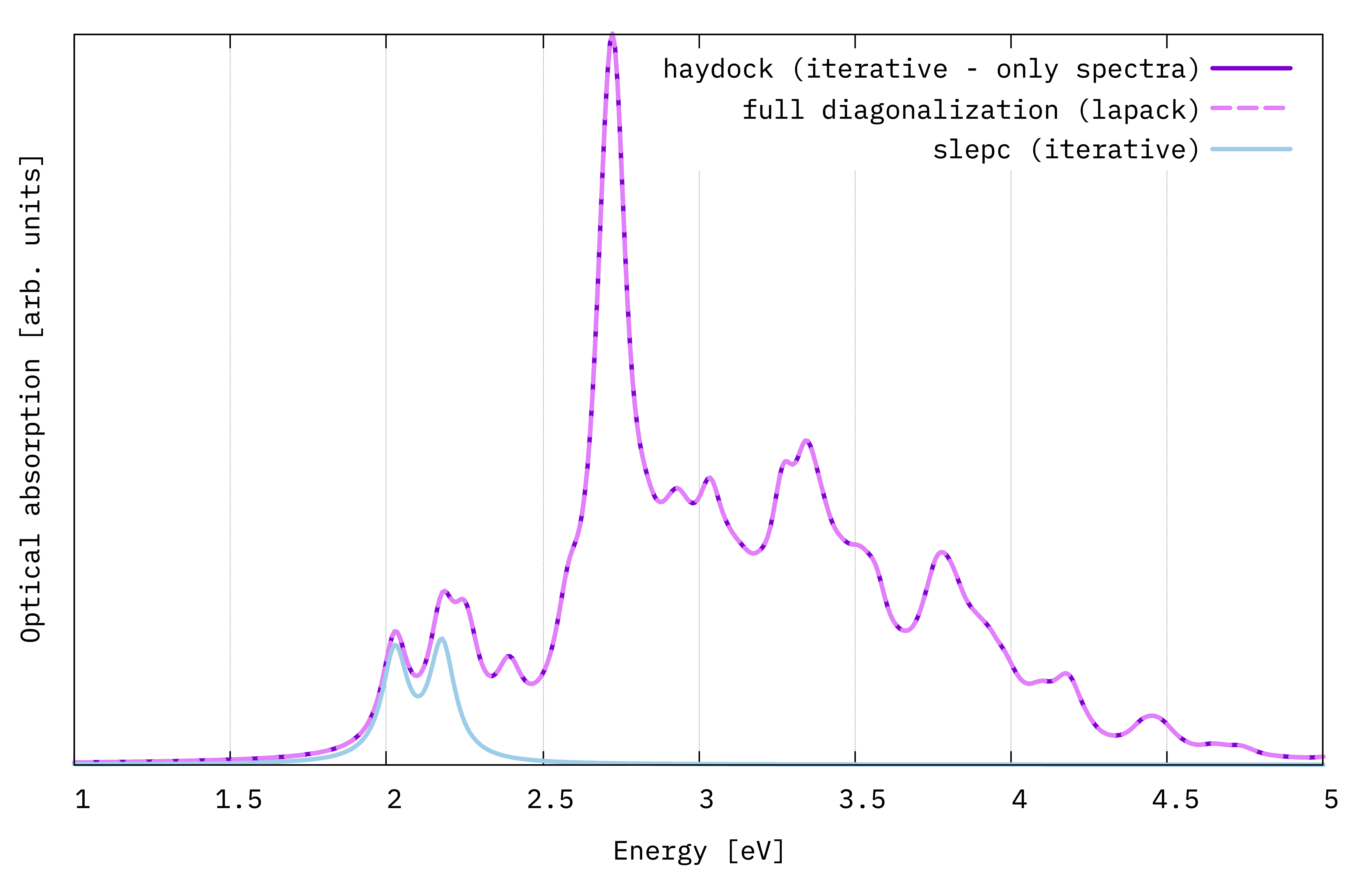
BSE optical absortion spectra of monolayer MoS2 obtained with three different diagonalization schemes.
This spectra are far from being numerically converged, but we can already see the main excitonic features of MoS2: two initial peaks at low energy (A and B exciton - the energy difference between them depends on the strength of the spin-orbit interaction) and a large resonance at higher energy, above the quasiparticle band gap.
Furthermore, we see that the haydock and diago solutions basically coincide. The slepc solution, given that we included only the first 10 states, will cut the spectrum off when they run out: here only the first two peaks are reproduced.
Note
We should study the slepc solver more. Try to increase BSSNEig and replot to check how it gradually reproduces a larger part of the full spectrum. Typically, you only need the spectrum in the low-energy window, and you don’t need to include many eigenvalues. If you don’t know where to start, try with 10% of the total size of the BSE kernel, which is usually both very fast and enough.
Now check the timings of the three methods from the report files:
$ grep "Timing " absorption_*/r-*
Clearly, there is a large difference between the full diagonalization and the iterative solvers.
Postprocessing: plotting the exciton wavefunction in real space
The wavefunction \(\Psi\) corresponding to the exciton with state index \(\lambda\) is constructed by linear combination of the electron and hole Bloch functions \(\phi\) via the excitonic eigenvector coefficients:
Here, \(\mathbf{r}_e\) and \(\mathbf{r}_h\) denote the electron and hole positions, respectively. It is not possible to fully visually represent this function because it depends on six variables. However, we can simplify it by fixing the hole at a certain chosen position (\(\mathbf{r}_0\)) and plotting the resulting function of the electron position only (we plot the intensity, which is real):
You can understand the meaning of \(N_\lambda(\mathbf{r}_e)\) as the conditioned probability of finding an electron at position \(\mathbf{r}_e\) given that the hole is fixed at \(\mathbf{r}_0\) for electron-hole state \(\lambda\).
Tip
How to choose \(\mathbf{r}_0\) in a meaningful way? This in general depends on what you want to visualize, but a good strategy is to fix the hole in the most “physically sound” position: this would be the position where the most important valence orbital contributing to exciton \(\lambda\) (i.e. the \(\phi_{vk}\) for which \(A^\lambda_{cvk}\) is maximum) has a maximum in intensity.
We will use the postprocessing executable ypp to get the exciton wavefunction.
Tip
You can do this also with Yambopy.
Go to the 03_BSE_wavefunction folder and create symbolic links to all the previously computed databases:
$ cd ../03_BSE_wavefunction/
$ ln -s ../01_BSE_Hamiltonian/SAVE/ .
$ ln -s ../01_BSE_Hamiltonian/GW_bnds/ .
$ ln -s ../01_BSE_Hamiltonian/BSE/ .
$ ln -s ../02_BSE_diagonalization/absorption_slepc/ .
The latter one contains the database ndb.BS_diago_Q1 with the exciton coefficients \(A^\lambda_{cvk}\).
Let us now analyse the exciton energies and their optical oscillator strengths (i.e., peak intensities in the spectrum).
Type
$ ypp -e s -J absorption_slepc,BSE,GW_bnds
Attention
You may need open an interactive session to run ypp. In this case remember to load the executables and pay attention to any run requirements.
You should obtain an output file ending in *_E_sorted.
Open it and inspect the data.
o-absorption_slepc.exc_qpt1_E_sorted
[...]
# Atom 1 with Z 42 [cc]:-0.295004043E-8   3.40641356      0.00000000
# Atom 1 with Z 16 [cc]:  2.95004058      1.70320678      2.93654299
# Atom 2 with Z 16 [cc]:  2.95004058      1.70320678     -2.93654299
#
#    Maximum Residual Value =  0.86686E-01
#
#    E [ev]             Strength           Index
#
     2.0163708         0.66523766E-10      1.0000000
     2.0171168         0.12820390E-10      2.0000000
     2.02876091        0.902098060         3.00000000
     2.02876735        0.857971907         4.00000000
     2.1630719         0.53834254E-09      5.0000000
     2.1630721         0.60582754E-10      6.0000000
     2.17986917        0.913443565         7.00000000
     2.17987561         1.00000000         8.00000000
     2.2404346         0.34227418E-09      9.0000000
     2.24088478        0.340123241E-8      10.0000000
[...]
Here we find the energies of the 10 exciton states we computed in the previous section with slepc (first column) and their corresponding optical strength (second column).
We can immediately notice two things. First, all the excitons found here are doubly degenerate: this is a consequence of the rotation symmetry of the hexagonal MoS2 crystal lattice.
Second, the first degenerate pair does not couple with light (a consequence of its spin-triplet structure): it’s a dark exciton. The excitons corresponding to the first two peaks seen in absorption are the (3-4) and (7-8), respectively.
Therefore, we will try to plot the wavefunction of excitons (3-4). Yambo will automatically recognize the degeneracy and sum the components accordingly.
To generate the ypp input file for the exciton wavefunction type
$ ypp -e w -F ypp_wfc.in
(as with yambo, you can see all the available options with ypp -h; here -e w stands for exciton wavefunction).
Open the resulting input file and modify the variables as shown. Try to think about the meaning of runlevels and variables as explained in the comments. Change the following variables as shown here:
excitons                         # [R] Excitonic properties
wavefunction                     # [R] Wavefunction
Format= "x"                      # Output format [(c)ube/(g)nuplot/(x)crysden]
Direction= "123"                 # [rlu] [1/2/3] for 1d or [12/13/23] for 2d [123] for 3D
FFTGvecs=  40            Ry      # [FFT] Plane-waves
#NormToOne                       # Normalize to one the maximum value of the plot
States= "3 - 3"                  # Index of the BS state(s)
BSQindex= 1                      # Q-Index of the BS state(s)
Degen_Step= 0.010000       eV    # Maximum energy separation of two degenerate states
% Cells
 12 | 12 | 1 |                   # Number of cell repetitions in each direction (odd or 1)
%
% Hole
 1.475 | 2.555 | 1.468 |         # [cc] Hole position in unit cell (positive)
%
We have selected the third exciton state in the list of States.
The Cells variable represents the extension in real space we want to consider in the calculation.
In MoS2, excitons have a large Bohr radius so we need to use a large number of repeated unit cells.
Finally, we need to set the hole position \(\mathbf{r}_0\).
We want to fix it in the middle of a Mo-S bond.
How do we do that?
Check again the previous *E_sorted file:
[...]
# Atom 1 with Z 42 [cc]:-0.295004043E-8   3.40641356      0.00000000
# Atom 1 with Z 16 [cc]:  2.95004058      1.70320678      2.93654299
# Atom 2 with Z 16 [cc]:  2.95004058      1.70320678     -2.93654299
[...]
These are the atomic positions in the unit cell in Cartesian coordinates. We can easily compute the midpoint between the first atom (Z=42, Mo) and the second (Z=16, S).
Finally, let’s submit the input with the script run_ypp.sh.
This will create a new directory EXC_WF.
At the end of the calculation, in there you will find the output file o-EXC_WF4.exc_qpt1_3d_3.xsf.
This can be visualized, for example, with the programs xcrysden or VESTA:
$ VESTA o-EXC_WF4.exc_qpt1_3d_3.xsf
You will see the atomic structure and the wavefunction intensity data represented as isosurface. After working on the figure layout, you should find something similar to this:
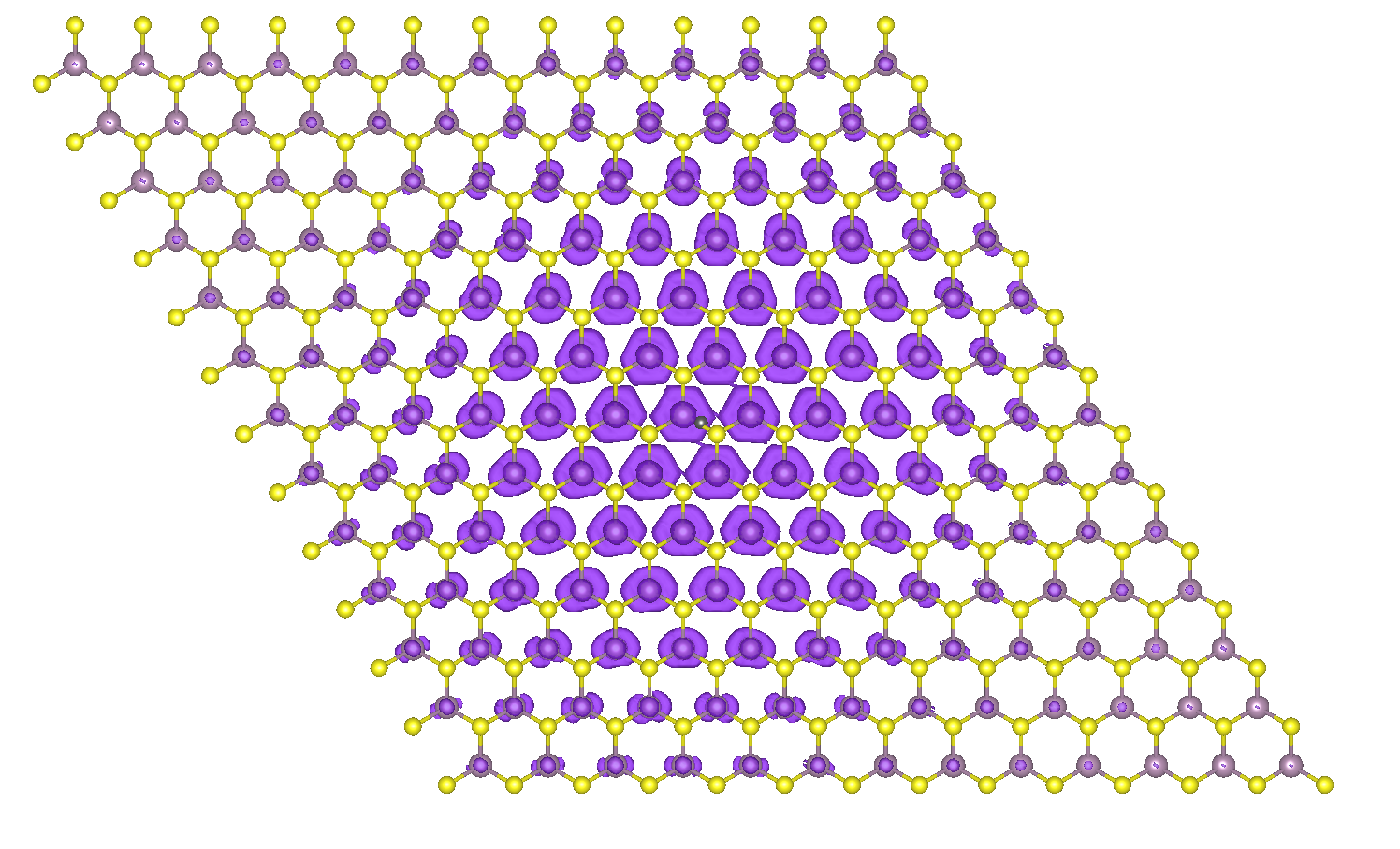
Electron density distribution for the first bright exciton of monolayer MoS2 with the hole fixed between the Mo-S bond.
Note that when the hole is fixed between a Mo-S bond, the relative eletron sits onto the Mo atoms. Try to inspect closely the shape of the isosurface on each atom: what does it remind you of? What does this shape suggest about the orbital character of the conduction electrons forming the bright exciton in MoS2?